An investigation of how normalisation and local modelling techniques confound machine learning performance in a mental health study

Abstract

Machine learning (ML) is increasingly deployed on biomedical studies for biomarker development (feature selection) and diagnostic/prognostic technologies (classification). While different ML techniques produce different feature sets and classification performances, less understood is how upstream data processing methods (e.g., normalisation) impact downstream analyses. Using a clinical mental health dataset, we investigated the impact of different normalisation techniques on classification model performance. Gene Fuzzy Scoring (GFS), an in-house developed normalisation technique, is compared against widely used normalisation methods such as global quantile normalisation, class-specific quantile normalisation and surrogate variable analysis. We report that choice of normalisation technique has strong influence on feature selection. with GFS outperforming other techniques. Although GFS parameters are tuneable, good classification model performance (ROC-AUC > 0.90) is observed regardless of the GFS parameter settings. We also contrasted our results against local modelling, which is meant to improve the resolution and meaningfulness of classification models built on heterogeneous data. Local models, when derived from non-biologically meaningful subpopulations, perform worse than global models. A deep dive however, revealed that the factors driving cluster formation has little to do with the phenotype-of-interest. This finding is critical, as local models are often seen as a superior means of clinical data modelling. We advise against such naivete. Additionally, we have developed a combinatorial reasoning approach using both global and local paradigms: This helped reveal potential data quality issues or underlying factors causing data heterogeneity that are often overlooked. It also assists to explain the model as well as provides directions for further improvement.

Biomarker; Data normalisation; Gene expression; Gene fuzzy scoring (GFS); Local modelling; Machine Learning; Mental health.

1. Introduction

1.1. Proper data normalisation is essential for biomedical data analysis

Biomedical data suffers from various sources of noise and biases: Other than biological variances due to different diseases or health conditions, there are unwanted variances generated during subject recruitment or experiment processes [1]. For example, systematic errors incurred during patient recruitment (e.g., biased subject recruitment procedure) may result in the sampled cohort being non-representative of the true disease population. Poorly controlled experimental conditions may also introduce unwanted variances among samples: Variable timings for specimen collection, inconsistent techniques for sample collection, and different storage conditions may lead to technical bias [2]. Following patient recruitment and sample collection, additional noise could be introduced when measuring biological signals. For example, when measuring gene expression using high-dimensional platforms such as microarrays, different temperatures, dyes or sample preparation procedures could lead to batch effects [1]. Such technical noise can be detected by data visualisation, or reduced/minimised via correction techniques such as data normalisation.

Data normalisation, in itself, encompasses a wide variety of data transformation techniques for removing non-biological variance in data [1]. Because many normalisation methods exist, selecting the most appropriate is difficult. Different techniques are developed to account for different types of technical noise, and many rely on certain assumptions. For example, Z-score normalisation requires the data to be normally distributed. Quantile normalisation, as one of the most popular normalisation techniques on microarray data, assumes all samples to have the same scale and distribution of gene expression [3]. Applying a normalisation technique without satisfying its assumptions may lead to distorted feature distributions or false differential gene reporting [4].

Among all normalisation techniques commonly used on gene expression data, Gene Fuzzy Scoring (GFS) is a new promising method proposed by Belorkar and Wong [5]. It is a rank-based method, which divides all genes into three regions based on the expression ranking within a sample. The highly expressed and lowly expressed genes are transformed into constant values, while the rest are transformed by a linear function based on their ranks. The method improves data quality by improving the signal-to-noise ratio with great interpretability. GFS also outperforms other common normalisation techniques for batch correction [5]. In GFS, grouping of genes within each sample is achieved by defining two percentile parameters ${\theta }_1$ and ${\theta }_2$, which were fixed at 5% and 15% in the original paper. Such tight thresholds come at high cost, leading to 85% of dimensionality reduction and information loss, which may cause us to miss important differentially expressed genes (DEGs), which are important for understanding how the biological mechanisms works. Hence, in this paper, we explore if different GFS thresholds have any significant impacts on DEG identification. Since GFS is in itself also a data normalization method, we would also like to study how GFS parameters affect the normalisation outcome and its concomitant impact on downstream machine learning.

1.2. Local modelling may have higher prediction power on heterogenous data

Besides normalisation techniques, the choice of machine learning (ML) paradigm may also affect the adaptability and explainability of a model. Usually, ML models are trained on all available samples. This is known as global modelling, which captures a broad view and selects important DEGs in the total sampled cohort [6]. However, global models may not generalise well on new samples, especially when the underlying population is highly heterogenous. For instance, for diseases with multiple subtypes, the genetic biomarkers could differ greatly among different subtypes. Such disease is not well summarised by a single global model.

Local modelling, in contrast, accounts for heterogeneity with better adaptability to new samples and higher degree of explainability [6]. As an instance of semi-supervised learning, local modelling first divides samples into subpopulations based on their similarity. Feature selection and model training are then performed within each subpopulation. Important features in one subpopulation may not be important for another. Theoretically, if the clustering is driven by biologically meaningful factors (such as disease subtypes, treatment received, etc.), local models have potential to be good predictors, and genes with high feature importance are likely to be signatures for the corresponding biologically meaningful subpopulation. Local modelling's superiority over global models on clinical datasets has been proven by its high accuracy when predicting 5-year survival outcome of lymphoma patients, a notoriously heterogenous disease [6]. However, we suspect that when data clustering is driven by other factors yielding non-biologically meaningful subpopulations, the consequent local models and gene signatures will be meaningless. Thus, inspecting the underlying factors contributing towards data heterogeneity is important for developing meaningful and interpretable local models. Instead of naively relying on either global models or local models alone, we propose leveraging both paradigms for comparative analyses. We reason this procedure is more insightful.

1.3. A case study on UHR clinical dataset

Ultra-high-risk (UHR) patients refer to young individuals with high risk of developing psychotic disorders [7]. Previous research has shown that early intervention targeting UHR patients not only manages current symptoms, but also prevents or delays the onset of psychotic disorders [7, 8]. Hence, early identification of UHR patients is crucial. Currently, diagnosis of UHR is done via a structured assessment known as The Comprehensive Assessment of At Risk Mental States (CAARMS), which is mainly based on risk factors and phenotypic syndromes, such as recent history of Attenuated Psychotic Symptoms (APS) and Brief Limited Intermittent Psychotic Symptoms (BLIPS) [7, 8, 9]. However, this method of diagnosis is likely to be flawed and usually leads to high false positive rates. Because the syndromes are nonspecific, and no full psychotic onset is observed on 50–90% of UHR patients within 12 months [10], more precise and accurate UHR diagnosis methods are required. One promising direction is to rely on genetic biomarkers revealing pathological linkage to psychotic onset.

To investigate UHR and psychosis, it makes sense to assay brain tissue directly. But this is not feasible in live people. Postmortem brain tissues have been used for many gene expression research of psychosis [11, 12]. However, this approach has many limitations: Brain tissue samples are very hard to retrieve, most of which are extracted after the subject is deceased. With the limited amount of samples, researchers have to deal with the transcriptional changes from prolonged duration of illness or medicine exposure [13]. Due to the invasive procedure, biomarkers identified in brain tissues can hardly be used for disease detection. Blood, as an alternative tissue source (surrogate tissue), is much more abundant, accessible, and less invasive to extract. Studies have shown that differential expression of genes in blood are correlated with pathological changes in the brain, despite the influences from other tissues [14]. Biomarkers found in blood are thus more generic, with greater potential for clinical applications [15].

1.4. Study objectives

Using a clinical dataset of UHR patients, we will study the impact of various normalisation techniques, including our in-house developed method GFS, on ML model performance. We are particularly interested in understanding how different GFS percentile thresholds (parameters) affect modelling results. Finally, we demonstrate how combining global and local modelling serves as a logic check for potential data quality issues or underlying factors of heterogeneity and provides means towards improving model explainability.

2. Materials and methods

2.1. Clinical datasets

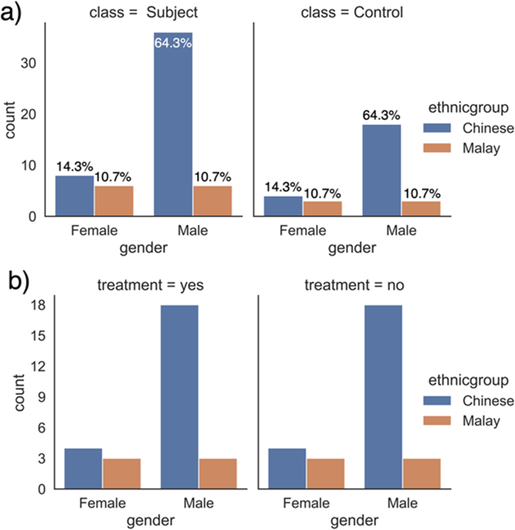
The main data used in this study was obtained from the Longitudinal Youth-at-Risk Study (LYRIKS) observational study [16]. The LYRIKS study aims to identify and assess the clinical, social, neuropsychological, and biological risk factors on an Asian UHR group of patients. Positive confirmation of UHR symptoms is based on the CAARMS diagnostic test. UHR cohort is compared against a control group of matched individuals in Singapore [16]. The data used in this study comprises 56 UHR subjects and 28 control subjects with balanced gender and ethnicity ratio across classes (Figure 1a). Half of the UHR patients have received psychosis treatment, while the other half and the healthy subjects have not been treated. Gender and ethnicity ratios are balanced between different treatment statuses among UHR patients as well (Figure 1b). Peripheral blood was sampled from the subject for gene expression measurement via microarray. Exact experimental procedure can be found in the previous study using the same dataset [4]. All samples were divided into training set and test set with a 3:1 ratio. Stratified sampling was applied during train-test split to ensure the same class ratio in both sets.

Figure 1.

Distribution of study subject information by a) class label (UHR vs Healthy), b) treatment statuses of UHR patients. Percentages (as insets in the plot) represent the proportionate breakdown of the total class counts. Both gender and ethnic groups have the same ratio in UHR and healthy group, and will likely not act as confounders. The gender and ethnic group distribution are the same for different treatment statuses among UHR patients as well.

To further study how GFS parameters may affect the analysis outcomes, two additional sets of microarray data were used as supplementary data (Table 1). The first contains gene expression data for Duschenne Muscular Dystrophy (DMD) patients and controls from Haslett et al. [17] and Pescatori et al. [18]. The second contains gene data for acute lymphoblastic leukaemia (ALL) patients and controls of acute myelogenous leukaemia (AML) from Golub et al. [19] and Armstrong et al. [20]. Both datasets were merged between two different studies using different microarray platforms. Only common genes detectable in both studies were retained post merging. For genes mapped to multiple probes (where each probe contains information on different parts of the same gene), the average values of the same-gene probes was taken.

Table 1.

Supplementary datasets to study the impact of GFS parameters on the gene signatures identified as well as the model performance.

	Source	Genes Retained	Class Distribution
DMD	Haslett et al. (2020)	8458	12 DMD +12 Control
	Pescatori et al. (2007)		22 DMD +14 Control
Leukemia	Armstrong et al. (2002)	5632	47 ALL +25 AML
	Golub et al. (1999)		24 ALL +24 AML

2.2. Microarray gene expression

Gene expression analyses is fundamental for genetics studies and can be used across a wide range of research purposes. E.g., we may understand changes in gene expressions associated with diseases which may lead towards better understanding and new therapies. Microarray, a popular and stable gene expression profiling method, can generate gene expression data for thousands of genes simultaneously. Leveraging on the tendency of complementary DNA strands to hybridize in a sequence specific. manner, microarrays contain thousands of short DNA strands (known as probes) corresponding to known genes, on which fluorescent-labeled samples can bind to. Based on the strength of fluorescent signal at each probe, researchers can measure gene expression strength. We used the Illumina HumanHT-12 v4 Expression BeadChip array with UHR data.

2.3. Normalisation techniques

Normalisation techniques such as global quantile normalisation (Global QN), class-specific quantile normalisation (Class QN), GFS [5] and Surrogate Variable Analysis (SVA) [21] were applied on the UHR dataset to study the impact of different normalisation techniques on machine learning model performance. For comparison, a non-normalised control group was constructed by applying natural log transformation to the dataset, which reduced the scale by ∼ 1000 times. All four normalisation techniques were applied on natural log transformed data.

Quantile normalisation (QN) is one of the most well-established normalisation techniques for high-dimensional biological data. It ranks the genes within each sample and substitutes gene expressions by the average values of genes with the same rank across all samples. Global quantile normalisation refers to applying QN across all samples regardless of their class labels. It is the default normalisation method for the Bioconductor Bioinformatics programming platform, and is very popular for use with microarray data and other high-throughput sequencing data [22]. Global QN assumes all samples to have similar scales and distributions of gene expression. The method has also been reported to drastically reduce the variances of true genetic expressions [23]. Hence, there is a risk of inter-class difference shrinkage after Global QN. In this scenario, it is recommended to apply class-specific QN to preserve the inter-class difference [24], which refers to applying QN separately for samples within each class. Class QN has been reported to be more robust in retaining actual class differences in the data than global QN [24]. However, as a supervised method, class-specific QN requires prior knowledge of class labels on test set as well. For both methods, test samples were normalised into the same space as the training samples for model performance assessment.

SVA is one of the most used methods for performing batch correction, especially when the source of batch-correlated variance is unknown (i.e., you do not know which samples belong to which batch). As a supervised method, SVA eliminates any other heterogeneity in the data except those due to the target class of interest by linear statistical modelling [21]. With prior knowledge of the class labels, the algorithm tries to identify other factors causing data heterogeneity by principal components, which are known as surrogate variables (SVs). Variances of SVs are then removed through regression modelling. Other than batch effect correction, SVA can also be used for data normalisation [4]. When normalising the test set, parameters of SVA algorithm were obtained from the training set, making sure the test samples were transformed into the same space as the training samples.

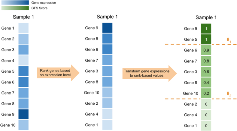
GFS is an unsupervised rank-based normalisation technique. With the pre-defined percentile thresholds of ${\theta }_1$ and ${\theta }_2$ , the genes are ranked in descending order within each subject. Values of all highly expressed genes in the upper ${\theta }_1$ percentile are set to 1, while values of all lowly expressed genes in the bottom $(1-{\theta }_2)$ percentile are set to 0. For genes with mid-level expression, the values are transformed by a linear function. Let $r(g_i,p_j)$ be the rank of gene $i$ in sample $j$, $q(p_j,\theta )$ be the rank of the upper $\theta$ percentile of genes, the GFS score $s(g_i,p_j)$ of gene $i$ in sample $j$ can be calculated as below [5].

$$s(g_i,p_j)=\{\begin{array}{ll}1\hfill & ifr(g_i,p_j)<q(p_j,{\theta }_1)\hfill \\ \frac{r(g_i,p_j)-q(p_j,{\theta }_2)}{q(p_j,{\theta }_1)-q(p_j,{\theta }_2)}\hfill & ifq(p_j,{\theta }_2)\ge r(g_i,p_j)>q(p_j,{\theta }_1)\hfill \\ 0\hfill & otherwise\hfill \end{array}$$

Essentially, GFS reduces the dimensionality by removing the lower $(1-{\theta }_2)$ percentile of genes of each sample. The two parameters ${\theta }_1$ and ${\theta }_2$ are essential in determining the amount of information to be removed. According to the original paper by Belorkar and Wong [5], ${\theta }_1$ and ${\theta }_2$ were set to be 5% and 15%, leading to 85% of the features being removed. It is unknown if these values are generalisable for any datasets. Hence, with ${\theta }_1$ fixed at 5% and 15%, the value of ${\theta }_2$ was altered to study its impact on the UHR dataset. ${\theta }_1$ and ${\theta }_2$ were also set to be 0% and 100%, when GFS resembled a rank-based min-max normalisation. When comparing GFS with other normalisation techniques, ${\theta }_1$ and ${\theta }_2$ were fixed at 5% and 15% respectively for consistency. Figure 2 below shows the working principle of GFS.

Figure 2.

Illustration of GFS on a single sample with 10 genes. Genes are first ranked based on expression level within the sample, which were then converted to GFS score based on ${\theta }_1$ and ${\theta }_2$ selection.

2.4. Feature selection

After data normalisation, feature selection was performed to select the significant genes to distinguish UHR and healthy subjects using the Boruta algorithm [25]. Boruta is a wrapper method to select useful features by comparing the feature importance between the original features and their random shuffles. Unlike other feature selection methods such as recursive feature elimination (RFE), Boruta does not require any parameter specification. For example, specifying the elimination step size and total number of features are required when using RFE. However, such information is usually unknown, as it is unsure how many genes are differentially expressed between the classes of interest. In this study, Boruta was applied as a wrapper with random forest classifier (RFC) with 500 iterations and a significance level of 5%. During each iteration, feature values were shuffled in each column, which was used to train an RFC model. An RFC model was trained using the original data before shuffling as well. Then, feature importance was compared. If a shadow feature with randomly shuffled values had lower feature importance than its original version, the feature was considered as a hit. If the feature had no hits after many iterations, then it was rejected as a non-significant feature for the target class differentiation. On the contrary, genes that outperformed its randomly shuffled copies repetitively were confirmed as significant features for the classification. It is worth noticing that the selection procedure suffered from multiple testing problem twice: One was testing of multiple genes during each iteration, and the other was testing the same gene for multiple times across iterations. This may lead to false positive genes being selected. A two-step correction was thus implemented. The first step targeted at the correction within each iteration using the less stringent Benjamini - Hochberg method [26]. The second step was to correct for multiple iterations over the same gene using Bonferroni method [27].

During feature selection process, only training set was used. The test set was then filtered by the selected features for model validation.

2.5. Machine learning modelling and feature importance

With the selected features, four different models were trained using the data with different normalisation techniques to cover a range of different model structures, namely random forest classifier (RFC), support vector machine classifier (SVC), Gaussian Naive Bayesian classifier (GNB) and gradient boosting classifier (GBoost). Model parameters were optimised via random search to achieve the best performance possible. To evaluate the model performance, area under the receiver operator characteristic curve (ROC - AUC) were used on test data. Because there were twice as many UHR subjects as healthy subjects in both training and test set, using metrics like accuracy may be misleading when the model had good performance on the majority class (i.e., UHR) but was incapable of classifying the minority class (i.e., healthy control) accurately.

Feature importance can be retrieved out of the box for tree-based models using scikit-learn package [28], which is based on the impurity reduction in the leaf nodes. More important features lead to more drastic impurity decrease in leaf nodes after branching. For other models where feature importance cannot be measured directly, the permutation importance was used instead. Permutation importance for each feature was calculated by the model performance decrease trained using the randomly shuffled version of the feature. If the feature is very important (i.e., has large contribution to the class differentiation), it is expected for the model performance to drop significantly after its values are randomly shuffled.

If a gene was part of the top 50% most important features in all models, it was considered a reproducible gene biomarker. False positive biomarkers identified were not expected to have reproducibly high contribution in different models. Correlation of selected genes with target class labels as well as other factors (i.e., gender, ethnic group, treatment, full psychosis conversion and age) were also evaluated to validate confounding effect by Mann Whitney U test with Benjamini - Hochberg correction or Pearson's correlation. Literature research was conducted to verify the biological linkage of the selected genes with UHR or psychosis. To validate if the model performance was due to true gene signatures or purely by chance, 1000 RFC models were trained using randomly selected gene signatures. Model reproducibility was defined as the probability of the random models having better performance than the one trained with selected genes. A highly reproducible model suggests that it is likely to generate equally good model performance using random features. The gene signatures selected are likely to be false and are no better than any random genes [29, 30].

2.6. Local modelling

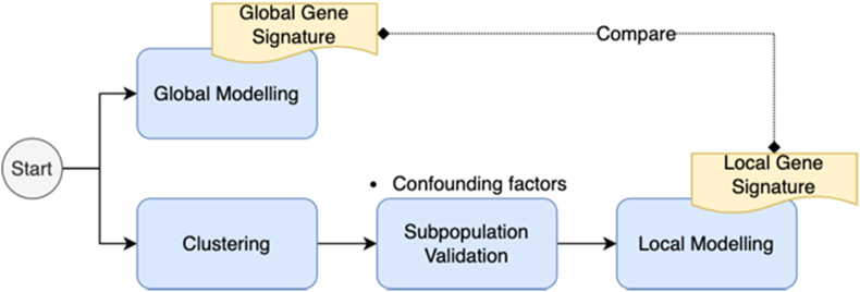
Local modelling is a semi-supervised technique for identifying locally significant features for class separation based on a subpopulation of the samples (i.e., a local cluster of samples). The training set was first transformed into Principal Components (PCs) with more than 85% variance coverage and divided into clusters using K-Means, where the number of clusters was determined based on elbow plot and silhouette scores. Feature selection was then conducted using Boruta to identify significant local gene signatures in each subpopulation, which were then used to train a local RFC model. To predict the class label of samples in test set, the test samples were first transformed into the same PC space as training set for dimensionality reduction. Then, based on the shortest Euclidean distance to cluster centroids, cluster membership was determined. The class label was predicted using the local model trained in the corresponding cluster. Due to the imbalance class distribution, local model performance was evaluated using ROC-AUC too. Figure 3 illustrates the high-level process of how results of global modelling and local modelling have been compared together.

Figure 3.

Illustration of how global modelling and local modelling are combined to reveal otherwise-hidden insights from the data.

3. Results

3.1. GFS outperforms other normalisation techniques in ML model performance

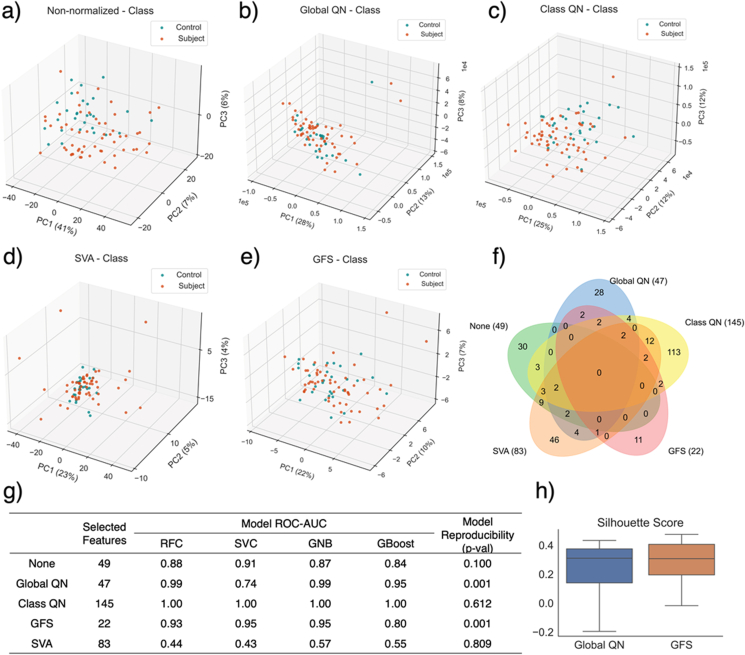
Normalisation techniques have strong impact on the differential genes identified as well as the classification model performance. Figures 4a – 4e shows the sample distribution on the first 3 PCs with various ormalization techniques prior to feature selection. Class QN provides the best discrimination between classes. However, the great separability observed is due to data leakage, as the class label is provided during the normalisation process. Samples with different class labels are normalised into separate spaces using class QN. The other supervised normalisation technique, SVA, shows the worst class separability, as all samples are clustered together with a few obvious outliers of UHR subjects. Model performance after SVA is also the worst, performing even lower than the non-normalised control group (Figure 4g). However, when coupled with other normalisation techniques, machine learning performance of SVA increased significantly to 0.94 (ROC-AUC of RFC model after Global QN and SVA). In practice, both Class QN and SVA cannot be used for classification modelling purposes, which is also demonstrated by the high p-values of model reproducibility (Figure 4g), indicating a model trained using randomly selected genes is very likely to have better performance than the model with selected gene features (reproduction probability of 61.2% and 80.9% for class QN and SVA, respectively). Further statistical test reveals that after class QN, 62% of the genes are reported to have p-values lower than 0.05 against the class labels. It is impossible that all these genes are differentially expressed between UHR and healthy subjects. Such high ratio of significant genes likely contains many false positives due to the leaky normalisation technique (These should not be used in any machine learning task). Global QN and GFS tend to provide moderate class separability as visualised on the PCA plot, as the PCs were highly impacted by outliers. However, after feature selection, classification models show good performance with low probability to reproduce (0.1% for both techniques). If samples are clustered by their class labels, silhouette scores after GFS normalisation tend to be slightly higher than those after Global QN (Figure 4h). This could be due to the tendency of inter-class difference shrinkage after Global QN. However, such shrinkage could be offset by machine learning, causing the model performance after Global QN to be slightly better than that after GFS. Therefore, GFS outperforms other normalisation techniques to some degree (on this dataset).

Figure 4.

Distribution of samples on PCA plots with the first 3 PCs after a) natural log transformation (non-normalised data), b) Global QN, c) class QN, d) SVA, and e) GFS with ${\theta }_1$ = 5% and ${\theta }_2$ = 15%. f) Venn diagram comparing the intersection of gene signatures identified by Boruta with different normalisation techniques. No common signatures were found using all four techniques or non-normalised control, indicating the high impact of data normalisation techniques on gene signature identification. g) Model performance measured by ROC - AUC with various normalisation techniques. GFS shows the best and most stable model performance. The model reproducibility refers to the probability of a RFC model trained using randomly selected N features having higher ROC - AUC than that of the selected features, where N is the number of selected features by Boruta. Global QN and GFS show the lowest p-value, indicating that the selected gene features are more likely to have biological linkage to UHR and tend not to be substitutable. h) silhouette scores of samples after Global QN and GFS normalisation. Samples of the same class are considered to belong to the same cluster.

It is also worth noticing that there are no common gene signatures found using different normalisation techniques, indicating the major impact of normalisation on DEG identification. None of the selected genes are found to be correlated with other factors such as age, ethnic group, treatment status or full conversion of psychosis.

3.2. GFS thresholds show little impact on model performance

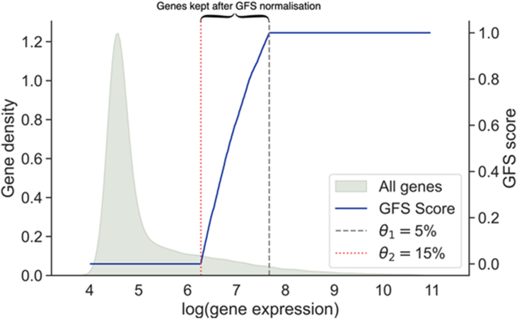
In the original GFS paper, the two thresholds ${\theta }_1$ and ${\theta }_2$ were fixed at 5% and 15% respectively, with good performance when separating samples from different batches with different diseases [5]. However, this parameter setting leads towards 85% information loss. It is uncertain if these default threshold settings can be extended to other dataset with equivalently good performance. Hence, the classification model performance was tested with various ${\theta }_1$ and ${\theta }_2$ values. Figure 5 visualises the amount of information retained from GFS normalisation with the example of ${\theta }_1$ = 5% and ${\theta }_2$ = 15%. Taking a random sample from the UHR dataset, distribution of gene expression is heavily right skewed after natural log transformation. For example, with ${\theta }_2$ = 15%, only genes with expression between the red dotted line and the grey dashed line are kept.

Figure 5.

Distribution of genes kept after GFS normalisation. Only genes between the lines are kept, whereas genes on the right side of the ${\theta }_1$ line or on the left side of the ${\theta }_2$ line are transformed into 1 or 0, respectively. Values of ${\theta }_1$ and ${\theta }_2$ were based on original GFS paper, which claimed to have good performance on separating samples from different batches with different diseases.

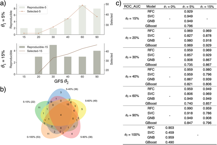
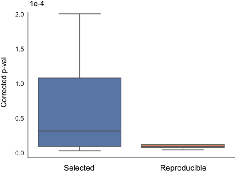
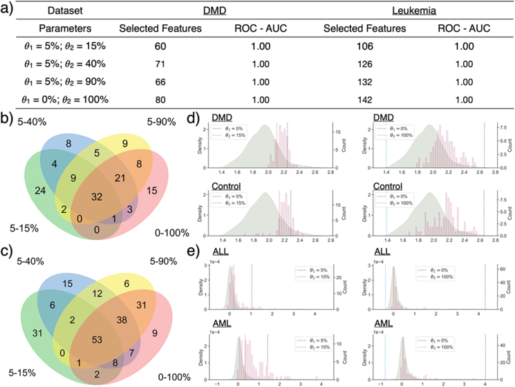
With different ${\theta }_2$ values, feature selection was done by Boruta, and machine learning models were trained using the selected features. As shown in Figure 6a, the number of selected features increases with increasing ${\theta }_2$ (i.e., more relaxed thresholds) while the value of ${\theta }_1$ is fixed. The number of genes found to be significant in multiple models also shows an increasing trend with ${\theta }_2$, especially when ${\theta }_1$ is fixed at 5%. Furthermore, with fixed ${\theta }_1$ and ${\theta }_2$, p-values associated with such reproducibly significant genes are lower than those of selected genes, which suggests those reproducible genes as more likely to be true genetic biomarkers of UHR (Figure 7). Similarly stable results were also obtained for the leukemia and DMD datasets (see Figure 8).

Figure 6.

a) Number of selected genes and reproducible genes given different GFS parameters. “Reproducible-5” refers to the number of reproducible genes with ${\theta }_1$ = 5%, and ${\theta }_2$ values are noted on x-axis in percentage. b) Venn diagram of selected genes with different GFS parameters. “5–15%" refers to ${\theta }_1$ = 5% and ${\theta }_2$ = 15%. c) Model performance with different GFS parameters measured by ROC - AUC. Regardless of the GFS parameter used, the model performance is consistently good with high ROC- AUC above 0.9 (RFC models).

Figure 7.

Distribution of p-values against class labels of selected genes and reproducible genes when ${\theta }_1$ = 0% and ${\theta }_2$ = 100%.

Figure 8.

a) Selected features and model performance in ROC - AUC in DMD dataset and Leukemia dataset. Like the UHR dataset, the model performance is stable across various GFS parameters, while the number of selected genes increases with more relaxed thresholds. b) Venn diagram of selected genes with various GFS parameters in DMD dataset and c) Leukemia dataset. d) Distribution of selected genes in DMD samples and healthy controls when ${\theta }_1$ = 5% and ${\theta }_2$ = 15% as well as ${\theta }_1$ = 0% and ${\theta }_2$ = 100%, respectively. Density plot in green represents the distribution of all genes, while histogram in pink represents the distribution of selected genes after GFS normalisation. Median of the selected gene expression is higher than that of all genes, indicating the gene signatures correlates with DMD tend to have relatively high expression level comparing to other genes. e) Distribution of selected genes in ALL subject and AML subject with ${\theta }_1$ = 5% and ${\theta }_2$ = 15% as well as ${\theta }_1$ = 0% and ${\theta }_2$ = 100%, respectively.

When comparing the signature genes identified with different thresholds, many genes are found repetitively, including four that are common to all ${\theta }_2$ values (Figure 6b, ARID4B, LOC401152, PTPRC, TRA2A with fixed ${\theta }_1$ of 5%). These are also found to be genes with high feature importance in multiple models. All four genes have been shown to have biological association with psychosis or mental disease. ARID4B has been reported to be part of a gene set with high expression variability in schizophrenia subjects [31]. Despite lack of study of direct correlation with psychosis, expression of LOC401152 in peripheral blood is down-regulated in bipolar patients treated with moderate dosage of lithium [32]. Glatt et al. [33] identified PTPRC as an alternatively spliced biomarker for schizophrenia and bipolar disorder patients in blood, and Nishioka et al. [34] reported TRA2A to be correlated with multiple indicators to measure the severity of schizophrenia.

Moreover, there are signature genes unique to certain levels of ${\theta }_2$. However, the difference in signature genes does not affect model performance. With different values of ${\theta }_1$ and ${\theta }_2$, the model performance for RFC and GNB remains around 90%–95% with minor fluctuations. ROC - AUC of SVC and GBoost are slightly lower, fluctuating around 80%–85% (Figure 6c). Because GFS only considers the ranking of gene expression within each sample, which is independent from the differential expression across classes. A gene signature with high differential expression across samples could be lowly expressed comparing to other genes from the same sample. It is not guaranteed that all DEGs are concentrated in a certain range of percentile within a sample. To verify the statement, ${\theta }_1$ and ${\theta }_2$ were set to 0% and 100%, respectively. With all genes transformed linearly by a rank-based min-max normalisation, 53 signature genes are found in total, out of which more than 80% were found with less relaxed thresholds.

The same experiment was repeated on DMD and Leukemia dataset with the same outcome. More signatures are identified with more relaxed ${\theta }_1$ and ${\theta }_2$ thresholds. Performance of RFC models is stable at ROC - AUC of 1.00 regardless of ${\theta }_1$ and ${\theta }_2$ values. Note that gene expressions for samples in DMD dataset are more normally distributed than those in UHR dataset, indicating that good performance with various GFS parameters can be generalised regardless of the gene expression distribution. 32 signatures were commonly found with different GFS thresholds, which is about 40%–50% of all the signature identified. Besides, when ${\theta }_1$ and ${\theta }_2$ are not 0% and 100%, not all signatures are found within the upper ${\theta }_1$ to ${\theta }_2$ percentile. Some gene signatures with expression ranking across the thresholds are also included. For example, Q14693 is a significant gene signature identified in DMD dataset with ${\theta }_1$ = 5% and ${\theta }_2$ = 15%. Its expression is within the upper 5%–15% percentile in control subjects, while its ranking is below the upper 15% percentile in DMD subjects, indicating that the expression of Q14693 tends to be down regulated in DMD subjects.

3.3. Local models may not always have high classification power due to inconsequential subpopulation

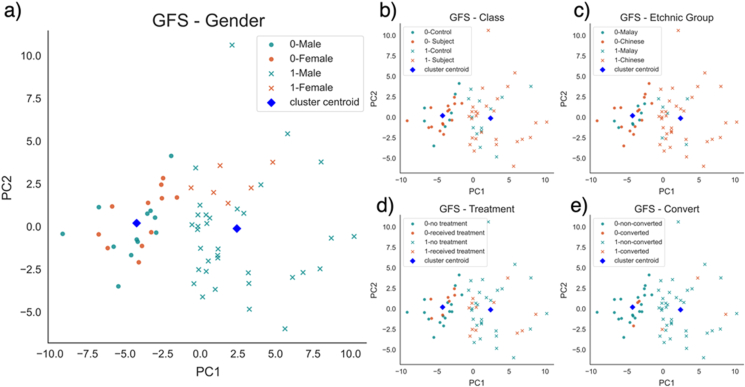
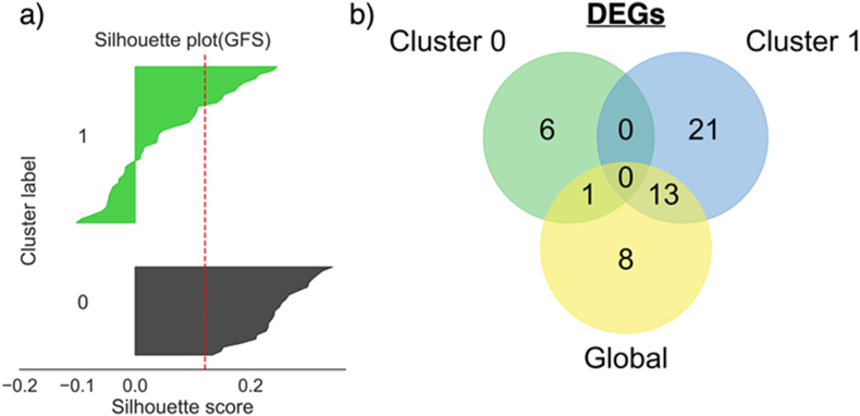
Due to the heterogeneous nature of UHR samples [4], global modelling may not have the best generalisability to new individual samples. If multiple biologically meaningful subpopulations are observable, local modelling with feature selection for each subpopulation is expected to yield more meaningful outcome. However, despite the attractiveness of such obvious reasoning, this is shown to be false on the UHR dataset. Class QN is omitted from the comparison, as samples within the same class tends to cluster together due to class label leakage during normalisation. After K-means clustering on the training data, it is observed that the clustering was dominantly driven by gender differences on PCA plots (Figure 9a shows one example after GFS normalisation). This is also validated by the chi-square test. When testing against cluster labels, only p-value of gender (4.58%) is lower than 5% after GFS normalisation, indicating association between the two variables. Other factors like UHR class labels, ethnic groups, treatment status, and full psychosis conversion status show no relationship with cluster labels (Figures 9b - 9e, p-values after GFS normalisation are 99.88%, 34.3%, 100%, and 91.72%, respectively). Since there is no known gender-specific differential gene expression between UHR subjects and healthy subjects in peripheral blood, it is hard to conclude the subpopulations are biologically meaningful. Besides, the boundary of subpopulations is not perfect, as the silhouette scores of many samples are negative (Figure 10a), indicating that they are closer to the other cluster than the one they belong to. Hence, samples within the same subpopulations may still be heterogenous.

Figure 9.

Subject distribution within each subpopulation after GFS normalisation (${\theta }_1$ = 5%, ${\theta }_2$ = 15%) by a) gender, b) class (Subject refers to UHR subject), c) ethnic group, d) treatment status, e) full psychosis conversion. Legends of the plot are in the format of “cluster - label” (e.g. “0-Male” refers to male subjects in cluster 0).

Figure 10.

a) Silhouette plot of samples after GFS normalisation (${\theta }_1$ = 5%, ${\theta }_2$ = 15%). Silhouette scores of some subjects in cluster 1 are negative, indicating that they are closer to cluster 0. b) Venn diagram of gene signatures found globally and locally per cluster. Global DEGs are heavily overlapping with DEGs from the male-dominant cluster 1, indicating the global signatures are skewed by male subjects as well.

Moreover, local models with locally selected features in general showed worse classification performance than the global models (Table 2). However, when supplying the local models with globally selected features, the model performance enhances regardless of the normalisation techniques (Table 2). It suggests that the local gene signatures are indeed inaccurate with lower representativeness than the global ones. When comparing the gene signatures identified locally and globally, a deeper overlap is observed between global signatures and local signatures from the male-dominant cluster 1 (Figure 10b). As there are twice more males than females in this dataset, it is not surprising that the global signatures are highly skewed by male subjects. Such insight could be easily missed if local modelling was not conducted. Furthermore, there is no common signatures found between the two local clusters, demonstrating the major impact of sampled population changes on the DEGs identified.

Table 2.

Number of features selected and model performance by local modelling, comparing to the model performance of local models with global features.

Normalisation Techniques	Local Model & Local Features			Local Model & Global Features
	Training cluster size	Feature Selected	RFC ROC-AUC	RFC ROC-AUC
None	34	22	0.765	0.857
	29	12
Global QN	29	46	0.745	0.857
	34	23
GFS (${\theta }_1$ = 5%, ${\theta }_2$ = 15%)	40	34	0.816	0.878
	23	7
SVA	18	4	0.459	0.531
	45	34

4. Discussion

4.1. GFS is a promising unsupervised sample-wise normalisation technique

GFS is a superior normalisation technique that boosts signal-to-noise ratio. The best classification performance is observed with GFS normalisation in both local and global modelling with ROC-AUC of 0.878 and 0.95, respectively. GFS is only dependent on the rank of gene expression within each sample instead of the sampled population. Hence, the outcome is consistent regardless of the population profile. On the contrary, the outcome of Global QN is highly dependent on the cohort profile, leading to different normalisation result of the same sample as the cohort changes. Another caveat of Global QN is that it is unable to preserve different distributions between biological classes, and the method forces all samples to have the same distribution after normalisation [35]. Such alterations in the distribution could lead to false discoveries of gene signatures in downstream analysis. Studies have also shown that the variance in gene expression tends to be reduced after Global QN, resulting in smaller inter-class differences [36].

SVA and Class QN, as supervised normalisation methods, should not be used with machine learning due to class leakage issues. Moreover, and particularly for SVA, the outcome of such supervised normalisation methods is heavily dependent on the labelling of the biological effects. Any biological difference not specified could be eliminated from the data, making it difficult for further data exploration [37]. These methods also suffer from reliance on the sampled cohort profile, hence the inconsistent normalisation outcome if the cohort changes. The poor class separability after SVA alone also suggests that when used for batch effect correction, SVA should be applied on normalised data to retain the biological differences in the data.

Therefore, selection of proper normalisation techniques is essential to develop interpretable machine learning models and accurate DEGs identification. Inappropriate normalisation methods may falsely exaggerate or minimise the level of inter-class gene expressions. The model may have good performance based on false gene signatures purely by chance with low biological interpretability [38]. In this regard, and on this dataset, GFS outperforms other normalisation methods.

4.2. With stable ML performance, relaxed GFS thresholds preserve more differentially expressed genes

The original GFS parameters selected were very stringent [5], leading to 85% of data loss. This is much more information loss than other differential expression algorithms like DESeq2, which also omit genes with very low expression levels [39]. In addition, with a more stringent set of parameters, the magnitude of differential expression could be erased as well. For genes with expression ranking across the thresholds (such as Q14693 in DMD dataset), it would be difficult to differentiate heavily down-regulated genes (with high log fold change between classes) from the moderately down-regulated ones (with low log fold change), as all low expressions have been erased to zero. It is found in this study that when coupled with feature selection, regardless of the GFS thresholds, machine learning models can accurately predict the sample classes on three different datasets. Hence, we would like to recommend selecting ${\theta }_1$ and ${\theta }_2$ dynamically, taking into consideration available computation power, desired dimensionality, and specific study objectives: A more relaxed set of thresholds naturally yields more gene signatures with less information loss, which might be used for DEG identification, whereas a more stringent set of thresholds might be sufficient to produce good performance for sample classification with less computation power.

4.3. Leveraging global and local models reveals the driven factors behind data heterogeneity

UHR samples are known to be heterogeneous [40]. Thus, local modelling might help reveal UHR subpopulations and their respective gene signatures. However, as demonstrated in this study, local modelling may not always be superior to global modelling when handling heterogenous data, which could be due to a few factors. Firstly, the subpopulation sizes are reduced after clustering. This might not be an issue when sample size is sufficiently large, whereas in this study, with only 63 samples to start with in the training set, such sample size reduction could be detrimental. With only 20–30 samples per subpopulation, the samples used for local gene signature selection are likely not representative enough of the general population profile. Thus, signatures selected locally tend to have lower prediction power, and local models might be overfitted.

In addition, the sample clustering is ostensibly, driven by gender. Although it is unknown if there is any gender-specific genetic biomarkers in peripheral blood, previous studies did suggest phenotypical and epidemical gender differences of schizophrenia [41, 42]. A few studies have also shown that proportion of male UHR patients transiting into psychosis or schizophrenia is higher [43, 44]. Male UHR or schizophrenia patients tend to show more negative symptoms than females. Note that such gender differences concluded from observational studies may be correlated with non-biological factors, such as sociological gender variances [45]. Despite gender-specific gene signatures have been identified in postmodern brain tissues for UHR and schizophrenia [46, 47, 48], whether such differential gene expression can be observed in peripheral blood tissues remains unknown.

The reciprocal inspection of global and local modelling serves as a logic check given presented data heterogeneity. Since there is no biological evidence to prove the subpopulations are meaningful, understanding what differentiates the two clusters is crucial for data quality assurance. For example, the possibility of batch effect or other unknown biases could not be simply ruled out for the UHR dataset. Since information about the sample collection methods and microarray batches is not available, it is unsure if samples in the male-dominant cluster (i.e., cluster 1) were handled by different lab technicians or on a different date. There might be other unknown gender-confounding factors that were not well controlled during the experiment. Furthermore, the gender ratio differences between clusters could also be due to the small sample size of atypical female subjects recruited. Further investigation is also required to validate the global gene signatures found on a larger dataset with balanced gender ratio, to ensure they are universal DEGs regardless of gender or other gender-confounding factors. Without comparing the result of global modelling and local modelling, the naïve analyst will not realise that the result might be distorted.

4.4. Limitations and future works

All three datasets used for GFS parameter tuning were generated from microarray platforms. To validate the generalisability of GFS normalisation on data from other platforms (e.g., RNA sequencing) or other omics data, the same set of experiments may be repeated on a variety of datasets. Besides, more clinical samples are required to study the biochemical correlations between the gene signatures found in peripheral blood with UHR, which is essential for diagnosing UHR accurately in a convenient and less painful way. Additionally, the sample size of the UHR dataset used in this study is relatively small, which may partially lead to the lack of representativeness in subpopulations after clustering. A larger dataset could be helpful to validate the effect of comparing global and local modelling results.

5. Conclusions

Normalisation techniques have essential impact on downstream data analysis, such as gene signature identification and the classification model performance. GFS, as a promising rank-based normalisation technique, can boost the signal-to-noise ratio in the data and produce stable gene signatures with high classification power. GFS is also robust, displaying stable performance even as its parameters were altered. Selecting more relaxed parameters increases differential gene identification. We recommend trying several GFS parameters to get a more dynamic understanding of the data. When analysing heterogeneous phenotypes, local models may not always outperform global models, especially when the subpopulations are not biologically or phenotypically meaningful. Reciprocal comparison of global and local modelling not only serves as a logic check of data heterogeneity and potential data quality issues, but also reveals more insights to improve model explainability.

Declarations

Author contribution statement

Xinxin Zhang: Conceived and designed the experiments; Performed the experiments; Analyzed and interpreted the data; Wrote the paper.

Jimmy Lee: Contributed reagents, materials, analysis tools or data.

Wilson Wen Bin Goh: Conceived and designed the experiments; Analyzed and interpreted the data; Wrote the paper.

Funding statement

This research/project was supported by the National Research Foundation, Singapore under its Industry Alignment Fund – Prepositioning (IAF-PP) Funding Initiative. Any opinions, findings and conclusions or recommendations expressed in this material are those of the author(s) and do not reflect the views of National Research Foundation, Singapore. This study was also supported by the National Research Foundation Singapore under the National Medical Research Council Translational and Clinical Research Flagship Programme (Grant No.: NMRC/TCR/003/2008) and a Ministry of Education (MOE), Singapore Tier 1 grant (Grant No. RG35/20).

Data availability statement

The authors do not have permission to share data.

Declaration of interests statement

The authors declare no conflict of interest.

Additional information

No additional information is available for this paper.

References

- 1.Scherer A. John Wiley & Sons; 2009. Batch Effects and Noise in Microarray Experiments: Sources and Solutions. [Google Scholar]
- 2.Karssen A.M., et al. Application of microarray technology in primate behavioral neuroscience research. Methods. 2006;38(3):227–234. doi: 10.1016/j.ymeth.2005.09.017. 03/01/2006. [DOI] [PubMed] [Google Scholar]
- 3.Kreil D.P., Russell R.R. Tutorial section: there is no silver bullet — a guide to low-level data transforms and normalisation methods for microarray data. Briefings Bioinf. 2005;6(1):86–97. doi: 10.1093/bib/6.1.86. [DOI] [PubMed] [Google Scholar]
- 4.Goh W.W.B., et al. Can peripheral blood-derived gene expressions characterize individuals at ultra-high risk for psychosis? eng, editor. Comput. Psychiatr. Psychol. 2017;1:168–183. doi: 10.1162/CPSY_a_00007. [DOI] [PMC free article] [PubMed] [Google Scholar]
- 5.Belorkar A., Wong L. GFS: fuzzy preprocessing for effective gene expression analysis. BMC Bioinf. 2016;17(17):540. doi: 10.1186/s12859-016-1327-8. 12/23 2016. [DOI] [PMC free article] [PubMed] [Google Scholar]
- 6.Kasabov N. Global, local and personalised modeling and pattern discovery in bioinformatics: an integrated approach. Pattern Recogn. Lett. 2007;28:673–685. 04/15. [Google Scholar]
- 7.Yung A.R. Treatment of people at ultra-high risk for psychosis. World Psychiatr. 2017;16(2):207–208. doi: 10.1002/wps.20424. (in eng) [DOI] [PMC free article] [PubMed] [Google Scholar]
- 8.McHugh M.J., et al. The Ultra-High-Risk for psychosis groups: evidence to maintain the status quo. Schizophr. Res. 2018;195:543–548. doi: 10.1016/j.schres.2017.09.003. 05/01/2018. [DOI] [PubMed] [Google Scholar]
- 9.Yung A.R., et al. Psychosis prediction: 12-month follow up of a high-risk (“prodromal”) group. Schizophr. Res. 2003;60(1):21–32. doi: 10.1016/s0920-9964(02)00167-6. 03/01/2003. [DOI] [PubMed] [Google Scholar]
- 10.Yung A.R., Nelson B. The ultra-high risk concept—a review. Can. J. Psychiatr. 2013;58(1):5–12. doi: 10.1177/070674371305800103. 01/01 2013. [DOI] [PubMed] [Google Scholar]
- 11.Duan J., et al. Transcriptomic signatures of schizophrenia revealed by dopamine perturbation in an ex vivo model. Transl. Psychiatry. 2018;8(1):158. doi: 10.1038/s41398-018-0216-5. 08/16 2018. [DOI] [PMC free article] [PubMed] [Google Scholar]
- 12.Sekar A., et al. Schizophrenia risk from complex variation of complement component 4. Nature. 2016;530(7589):177–183. doi: 10.1038/nature16549. 02/01 2016. [DOI] [PMC free article] [PubMed] [Google Scholar]
- 13.Sequeira P.A., Martin M.V., Vawter M.P. The first decade and beyond of transcriptional profiling in schizophrenia. Neurobiol. Dis. 2012;45(1):23–36. doi: 10.1016/j.nbd.2011.03.001. (in eng) [DOI] [PMC free article] [PubMed] [Google Scholar]
- 14.Jasinska A.J., et al. Identification of brain transcriptional variation reproduced in peripheral blood: an approach for mapping brain expression traits. Hum. Mol. Genet. 2009;18(22):4415–4427. doi: 10.1093/hmg/ddp397. [DOI] [PMC free article] [PubMed] [Google Scholar]
- 15.Lee J., Goh L.-K., Chen G., Verma S., Tan C.-H., Lee T.-S. Analysis of blood-based gene expression signature in first-episode psychosis. Psychiatr. Res. 2012;200(1):52–54. doi: 10.1016/j.psychres.2012.03.021. (in eng) 11//2012. [DOI] [PubMed] [Google Scholar]
- 16.Lee J., et al. The longitudinal Youth at risk study (LYRIKS) — an Asian UHR perspective. Schizophr. Res. 2013;151(1):279–283. doi: 10.1016/j.schres.2013.09.025. 12/01/2013. [DOI] [PubMed] [Google Scholar]
- 17.Haslett J.N., et al. Gene expression comparison of biopsies from Duchenne muscular dystrophy (DMD) and normal skeletal muscle. Proc. Natl. Acad. Sci. Unit. States Am. 2002;99(23):15000. doi: 10.1073/pnas.192571199. [DOI] [PMC free article] [PubMed] [Google Scholar]
- 18.Pescatori M., et al. Gene expression profiling in the early phases of DMD: a constant molecular signature characterizes DMD muscle from early postnatal life throughout disease progression. Faseb. J. 2007;21(4):1210–1226. doi: 10.1096/fj.06-7285com. 04/01 2007. [DOI] [PubMed] [Google Scholar]
- 19.Golub T.R., et al. Molecular classification of cancer: class discovery and class prediction by gene expression monitoring. Science. 1999;286(5439):531–537. doi: 10.1126/science.286.5439.531. [DOI] [PubMed] [Google Scholar]
- 20.Armstrong S.A., et al. MLL translocations specify a distinct gene expression profile that distinguishes a unique leukemia. Nat. Genet. 2002;30(1):41–47. doi: 10.1038/ng765. 01/01 2002. [DOI] [PubMed] [Google Scholar]
- 21.Leek J.T., Storey J.D. Capturing heterogeneity in gene expression studies by surrogate variable analysis. PLoS Genet. 2007;3(9):e161. doi: 10.1371/journal.pgen.0030161. [DOI] [PMC free article] [PubMed] [Google Scholar]
- 22.Qiu X., Wu H., Hu R. The impact of quantile and rank normalization procedures on the testing power of gene differential expression analysis. BMC Bioinf. 2013;14(1):124. doi: 10.1186/1471-2105-14-124. 04/11 2013. [DOI] [PMC free article] [PubMed] [Google Scholar]
- 23.Klebanov L., Yakovlev A. How high is the level of technical noise in microarray data? Biol. Direct. 2007;2(1):9. doi: 10.1186/1745-6150-2-9. 04/11 2007. [DOI] [PMC free article] [PubMed] [Google Scholar]
- 24.Zhao Y., Wong L., Goh W.W.B. How to do quantile normalization correctly for gene expression data analyses. Sci. Rep. 2020;10(1):15534. doi: 10.1038/s41598-020-72664-6. 09/23 2020. [DOI] [PMC free article] [PubMed] [Google Scholar]
- 25.Kursa M.B., Rudnicki W.R. Feature selection with the Boruta package. J. Stat. Software. 2010;36(11):1–13. 09/16. [Google Scholar]
- 26.Benjamini Y., Hochberg Y. Controlling the false discovery rate: a practical and powerful approach to multiple testing. J. Roy. Stat. Soc. B. 1995;57(1):289–300. http://www.jstor.org/stable/2346101 [Online]. Available: [Google Scholar]
- 27.Dunn O.J. Multiple comparisons among means. J. Am. Stat. Assoc. 1961;56(293):52–64. 03/01 1961. [Google Scholar]
- 28.Pedregosa F., et al. Scikit-learn: machine learning in Python. J. Mach. Learn. Res. 2011;12(null):2825–2830. [Google Scholar]
- 29.Goh W.W.B., Wong L. Why breast cancer signatures are no better than random signatures explained. Drug Discov. Today. 2018;23(11):1818–1823. doi: 10.1016/j.drudis.2018.05.036. 11/01/2018. [DOI] [PubMed] [Google Scholar]
- 30.Goh W.W.B., Wong L. Turning straw into gold: building robustness into gene signature inference. Drug Discov. Today. 2019;24(1):31–36. doi: 10.1016/j.drudis.2018.08.002. 01/01/2019. [DOI] [PubMed] [Google Scholar]
- 31.Huang G., Osorio D., Guan J., Ji G., Cai J.J. Overdispersed gene expression in schizophrenia. NPJ Schizophr. 2020;6(1):9. doi: 10.1038/s41537-020-0097-5. (in eng) [DOI] [PMC free article] [PubMed] [Google Scholar]
- 32.Beech R.D., et al. Gene-expression differences in peripheral blood between lithium responders and non-responders in the Lithium Treatment-Moderate dose Use Study (LiTMUS) Pharmacogenomics J. 2014;14(2):182–191. doi: 10.1038/tpj.2013.16. 04/01 2014. [DOI] [PubMed] [Google Scholar]
- 33.Glatt S.J., et al. Alternatively spliced genes as biomarkers for schizophrenia, bipolar disorder and psychosis: a blood-based spliceome-profiling exploratory study. Curr. Pharmacogenomics Personalized Med. (CPPM) 2009;7(3):164–188. doi: 10.2174/1875692110907030164. (in eng) [DOI] [PMC free article] [PubMed] [Google Scholar]
- 34.Nishioka M., et al. Comprehensive DNA methylation analysis of peripheral blood cells derived from patients with first-episode schizophrenia. J. Hum. Genet. 2013;58(2):91–97. doi: 10.1038/jhg.2012.140. 02/01 2013. [DOI] [PubMed] [Google Scholar]
- 35.Hicks S.C., Okrah K., Paulson J.N., Quackenbush J., Irizarry R.A., Bravo H.C. Smooth quantile normalization. Biostatistics. 2018;19(2):185–198. doi: 10.1093/biostatistics/kxx028. (in eng) [DOI] [PMC free article] [PubMed] [Google Scholar]
- 36.Bolstad B.M., Irizarry R.A., Åstrand M., Speed T.P. A comparison of normalization methods for high density oligonucleotide array data based on variance and bias. Bioinformatics. 2003;19(2):185–193. doi: 10.1093/bioinformatics/19.2.185. [DOI] [PubMed] [Google Scholar]
- 37.Jaffe A.E., et al. Practical impacts of genomic data “cleaning” on biological discovery using surrogate variable analysis. BMC Bioinf. 2015;16(1):372. doi: 10.1186/s12859-015-0808-5. 11/06 2015. [DOI] [PMC free article] [PubMed] [Google Scholar]
- 38.Abbas-Aghababazadeh F., Li Q., Fridley B.L. Comparison of normalization approaches for gene expression studies completed with high-throughput sequencing. PLoS One. 2018;13(10):e0206312. doi: 10.1371/journal.pone.0206312. [DOI] [PMC free article] [PubMed] [Google Scholar]
- 39.Love M.I., Huber W., Anders S. Moderated estimation of fold change and dispersion for RNA-seq data with DESeq2. Genome Biol. 2014;15(12):550. doi: 10.1186/s13059-014-0550-8. 12/05 2014. [DOI] [PMC free article] [PubMed] [Google Scholar]
- 40.Fusar-Poli P., et al. Heterogeneity of psychosis risk within individuals at clinical high risk: a meta-analytical stratification. JAMA Psychiatr. 2016;73(2):113–120. doi: 10.1001/jamapsychiatry.2015.2324. [DOI] [PubMed] [Google Scholar]
- 41.Falkenburg J., Tracy D.K. Sex and schizophrenia: a review of gender differences. Psychosis. 2014;6(1):61–69. 01/02 2014. [Google Scholar]
- 42.Seeman M.V. Gender differences in schizophrenia. Can. J. Psychiatr. 1982;27(2):107–112. doi: 10.1177/070674378202700204. 03/01 1982. [DOI] [PubMed] [Google Scholar]
- 43.Nordentoft M., et al. Transition rates from schizotypal disorder to psychotic disorder for first-contact patients included in the OPUS trial. A randomized clinical trial of integrated treatment and standard treatment. Schizophr. Res. 2006;83(1):29–40. doi: 10.1016/j.schres.2006.01.002. 03/01/2006. [DOI] [PubMed] [Google Scholar]
- 44.Ziermans T.B., Schothorst P.F., Sprong M., van Engeland H. Transition and remission in adolescents at ultra-high risk for psychosis. Schizophr. Res. 2011;126(1):58–64. doi: 10.1016/j.schres.2010.10.022. 03/01/2011. [DOI] [PubMed] [Google Scholar]
- 45.Rietschel L., et al. Clinical high risk for psychosis: gender differences in symptoms and social functioning. Early Interven. Psychiatr. 2017;11(4):306–313. doi: 10.1111/eip.12240. 08/01 2017. [DOI] [PubMed] [Google Scholar]
- 46.Bristow G.C., Bostrom J.A., Haroutunian V., Sodhi M.S. Sex differences in GABAergic gene expression occur in the anterior cingulate cortex in schizophrenia. Schizophr. Res. 2015;167(1-3):57–63. doi: 10.1016/j.schres.2015.01.025. (in eng) [DOI] [PMC free article] [PubMed] [Google Scholar]
- 47.de Castro-Catala M., Barrantes-Vidal N., Sheinbaum T., Moreno-Fortuny A., Kwapil T.R., Rosa A. COMT-by-sex interaction effect on psychosis proneness. BioMed Res. Int. 2015;2015:829237. doi: 10.1155/2015/829237. (in eng) [DOI] [PMC free article] [PubMed] [Google Scholar]
- 48.Mamoor S. 2020. GABARAPL1 Is Differentially Expressed in the Brains of Patients with Psychotic Disorders. [Google Scholar]
Associated Data
This section collects any data citations, data availability statements, or supplementary materials included in this article.