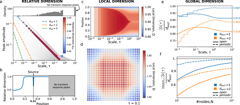
Fig. 1. The relative, local and global dimension.

a-c Line graph example with n = 500 nodes representing the interval [0, 1]. a The relative dimension of nodes given a source located at x = 0.33. The grey lines are the transient responses of the (non-source) nodes and the position of the peaks in the transient responses are highlighted by dots, coloured by their relative dimension. Top inset, a histogram of transient response peaks where the far right bin corresponds to nodes where no peak in the transient response was observed, and thus no relative dimension could be calculated. b The relative dimension as a function of position in [0, 1] shows a plateau near d_rel = 1 for nodes near the source. The grey region indicates the set of nodes for which no peak was observed. c The local dimension of each node as a function of scale, where above τ = 1, the stationary state is attained and the local dimension is stable. d The local dimension of the grid graph (n = 500) at scale τ = 0.1, showing inhomogeneities due to the boundaries similar to the line graph. e The evolution of the global dimension $\mathfrak{D}\left(\tau \right)$ (normalised by the expected Euclidean dimension) as a function of scale for the same line and grid graph as well as their periodic equivalent graphs, illustrating differing behaviours emerging from the influence of the boundaries or the topology. f For the same graphs as in e, we increase the number of nodes in each dimension to measure the convergence rate of ${\max }_{\tau }\mathfrak{D}\left(\tau \right)$ to the underlying Euclidean dimension d_eucl, showing a faster convergence for lower dimensional spaces and periodic grids.