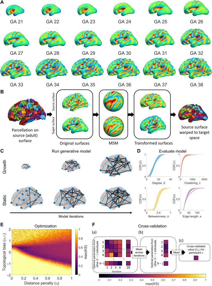
Fig. 1. Schematic of our approach to fitting and evaluating generative connectome models.
(A) Fetal surfaces from 21 to 38 weeks GA, showing sulcal depth. (B) To estimate how network wiring costs change through development, we parcellate the adult surface and use spherical MSM based on sulcal depth to map the parcellation to each of the fetal (target) surfaces. This procedure allows us to track the location of each parcellated region and estimate how wiring costs change through development. (C) Generative models were run using estimates of wiring cost based on adult distances (static models) or distances that change over time (growth models). (D) Benchmark topological properties were measured for each synthetic network and compared to the distributions of the empirical network using the KS statistic to quantify model fit (similar distributions indicate a better fit; thick lines represent empirical data, and lighter lines correspond to different realizations of a model). (E) Steps (C) and (D) were repeated for different parameter values in each model using an optimization scheme that searches the parameter landscape to find the parameter combination that yields the best fit to the data. Starting with an initial random sample, the algorithm narrows in on areas of the landscape associated with better fits and samples those regions more often (see Methods). (F) Leave-one-out cross-validation was used to avoid overfitting. For a given participant’s network, the best-fitting parameters for the 99 other participants are used to generate model networks. These models are iterated 20 times to account for the inherent stochasticity of the models (a), and the average across these 20 iterations is then taken to yield 99 fit values (b). These 99 fit values are then averaged (c), resulting in a single, cross-validated fit statistic, FCV, for each person.

