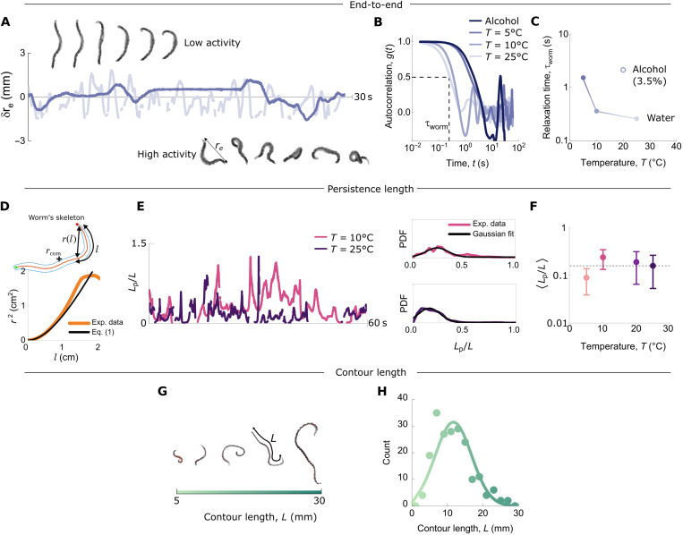
Fig. 1. Active worm characterization.

(A) Sequence of images of a single worm at a low level of activity (T = 5°C) compared with the same worm at a high level of activity (T = 25°C). The fluctuating end-to-end distance δr_e highlights the effect of the temperature on the activity [results from (32)]. (B) Autocorrelation function of δr_e (Eq. 3) at the different temperature T = 5°, 10°, and 25°C and in the presence of alcohol shown in (A), with the same color code. From this, the characteristic time τ_worm of a single worm was determined as indicated by the dotted lines and reported in (C) as a function of the temperature and in the presence of alcohol. (D) Persistence length L_p of a worm at a given temperature T and time t, determined by fitting the dependence of the end-to-end distance r(l) with the contour length l (Eq. 1). (E) Persistence length over 60 s for 3000 consecutive conformations (the shape is tracked at a frame rate of 50 fps). The corresponding probability distribution function is shown for two temperatures. From the latter, we extracted the persistence length (F) as a function of temperature by fitting a Gaussian distribution. Error bars are 1σ. (G) The contour length L of a T. tubifex worm increases with its age. (H) A typical distribution of contour lengths from the same batch of worms. The solid curve is a fit to a Gaussian distribution.