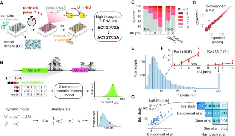
Figure 1.
cDTA-seq and genome-wide transcript half-life estimation. (A) cDTA-seq protocol outline. 4tU is added to dozens of quantified samples to label new RNA molecules. Cells are then immediately fixed with a pre-fixed constant amount of spike-in cells (K. lactis yeast in this case). RNA is extracted, 4tU is alkylated and RNA-seq libraries are prepared, resulting in T→C conversions where 4tU was incorporated. The entire process is performed in a 96 sample format. (B) Transcript-level analysis outline. Read conversion statistics per gene are fitted with a binomial mixture model to estimate the percent of recently-transcribed molecules (pr). Assuming a first-order kinetic model (C - number of cells, M—number of mRNA molecules,  are growth, production, and degradation rates respectively), and assuming steady-state, pr can be translated to transcript half-life given the known labeling period (t). See methods and supplementary material for more details. (C) 4tU conversion is effective, reproducible and measures transcription. Percent of reads (y-axis) along a 4tU time course (x-axis) with a different number of observed T→C conversions (legend, N = 6). Samples exposed to vehicle (DMSO) or the transcription inhibitor thiolutin for 15 min (and labeled with 4tU for 6 min, N = 2). Note that the y-axis begins at 75%, i.e. most reads have no conversions. (D) Binomial Mixture Model (BMM) fits the data. Read conversion statistics are fitted with a 2-component BMM. Each dot represents the number of reads with a certain number of observed Ts and T→C conversions (color as in E). x-axis is the expected number of reads for each (T,T→C) pair assuming the model and the observed #T distribution in the data, the y-axis is the observed number of reads in each (T, T→C) combination. Additional components do not improve the likelihood of the data (Supplementary Figure S1D). (E) Half-life distribution for all yeast transcripts. Assuming steady-state, transcript-specific and global parameters are iteratively fitted, resulting in the half-life of each transcript. The median of the distribution is 8.2', transcripts with a half-life of 45′ or longer are counted in the rightmost bin. (F) Examples of estimated pr along the time course. The individually estimated pr per time point and replicate (N = 6) for two transcripts (Pxr1 and Rpl34A) are shown as red dots along the time course. The data is fitted with a single parameter per gene (degradation rate) resulting in an estimate of 10.9’ half-life for Pxr1 and a 131’ half-life for Rpl34A. Using these estimates, the expected pr along the time course is plotted as a red line with 95% CI as a red shaded area. (G) Half-life estimates correlate with various studies. Half-lives from this and four other published studies are compared to each other and the linear explanatory value (R2) is denoted in the upper diagonal matrix. The scatter depicts a specific example of the comparison between this study and the rates from Baudrimont et al where estimates were not obtained by metabolic labeling.

