Limitations of machine learning models when predicting compounds with completely new chemistries: possible improvements applied to the discovery of new non-fullerene acceptors

Abstract

We try to determine if machine learning (ML) methods, applied to the discovery of new materials on the basis of existing data sets, have the power to predict completely new classes of compounds (extrapolating) or perform well only when interpolating between known materials. We introduce the leave-one-group-out cross-validation, in which the ML model is trained to explicitly perform extrapolations of unseen chemical families. This approach can be used across materials science and chemistry problems to improve the added value of ML predictions, instead of using extrapolative ML models that were trained with a regular cross-validation. We consider as a case study the problem of the discovery of non-fullerene acceptors because novel classes of acceptors are naturally classified into distinct chemical families. We show that conventional ML methods are not useful in practice when attempting to predict the efficiency of a completely novel class of materials. The approach proposed in this work increases the accuracy of the predictions to enable at least the categorization of materials with a performance above and below the median value.

We try to determine if machine learning (ML) methods, applied to the discovery of new materials on the basis of existing data sets, have the power to predict new classes of compounds or perform well only when interpolating between known materials.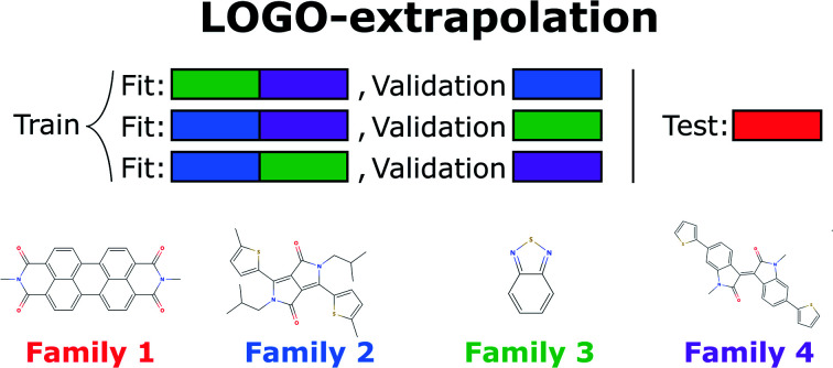

I. Introduction

One of the most exciting recent developments of materials discovery is the adoption of machine learning (ML) to guide the exploration of chemical and materials space.^1–4 In a typical application, existing datasets of experimental characterizations are often combined with computed features of the same materials and used to predict the property of interest of novel materials. The field is very frequently reviewed,^5–9 and some examples include alloys,¹⁰ polymers,¹¹ perovskites¹² and other inorganic solids.^13–18 Although the results are impressive and have prompted a widespread adoption of such methods across all areas of materials discovery, there is still some uncertainty over the ability of ML to explore completely new chemical/material spaces.¹⁹ In general, the predictive ability of ML is computed via cross-validation, i.e., predicting the performance of materials in a testing set that has not been included in the training set to optimize the ML algorithm, where training and testing sets are randomly generated from all data available in various ways. It is known that such algorithms perform better with larger data sets and with training data as close as possible to the ones to be predicted. Cross-validation generally gives the same weight to all predictions, whether they are for entries very close to existing ones in the training set (producing, in essence, an interpolation) or they are entirely novel (producing a much more challenging extrapolation). Moreover, materials are generally clustered by scientists into families based on their related chemical structures. Any discovery of a new family of compounds is regarded as a breakthrough, while discovering a novel member of an existing family is considered a more incremental advance. Therefore, accurate predictions within the families of known compounds and outside such families have a completely different value to the community. It should be noted that there are other non-random cross-validation methods, like scaffold-splits, time-splits and stratified-splits, which offer an alternative way to evaluate models. The general impact of such methods on the evaluation of the model can be found in ref. 20 and 21. Stratified sampling has also been used to train models in organic solar cells, although is has a minimal impact.²² In our preliminary work with this dataset, time-splits do not perform well, as the validation families are developed at similar points in time. Scaffold splits would use certain structural properties to split the data into groups, although here we opted for a combination of structural and electronic characteristics to categorize in groups, as explained in Section 3 of the ESI.†

The goal of this work is to assess the ability of ML to predict the efficiency of interesting energy materials from completely new families and offer a new method to do so. In this context, by completely new, we mean materials that belong to a chemical family that is not present when training the model, and can be generated using chemical intuition, database searching or generative models.²³ Then, one can use our methodology to screen these candidates and decide which ones will have a larger performance, reducing the number of candidates and accelerating the production of materials from new families. The methodology, in the most general terms, consists of constructing an ML model that is trained without any information on a new family of materials and assessing its quality in predicting the property of known elements of such family. Note that here we refer to training as the process of finding the optimum hyperparameters through a specific validation method. A practical problem is that the definition of “new” is not mathematically accurate, and the novelty of a material is related to (a combination of) electronic, geometric or synthetic features that cannot be captured by an algorithm, while they will appear as self-evident to any expert in the relevant scientific domain. The problem of predicting the target properties of data outside of the training domain is also often tackled with transfer learning, where a previously trained method is used a starting point when predicting data in a new domain. We chose to study the ability of ML to explore new chemical space in the context of predicting novel non-fullerene acceptors for organic solar cells (OSCs).^24–26 The topic is of significant contemporary interest as the identification of non-fullerene acceptors is considered essential to develop a competitive OSC technology and recent improvements have seen an almost three-fold increase in efficiency in five years since the report of non-fullerene electron acceptor (ITIC).^27,28 For this scientific problem, there are well-defined families of acceptors recognized by the community and used to categorize the recent advances in the field. We can, therefore, ask whether new families of non-fullerene acceptors could have been predicted without any information on any member of that family. In this work, we discuss how a conventional cross-validation results in an overoptimistic evaluation of models when they are eventually used to predict new classes of compounds. We aim to draw conclusions on the specific field of computer-aided discovery of OSCs acceptors but also, more generally, on a practical approach to assess the usefulness of ML methods for more exploratory research. There have been other recent studies that evaluate ML models with out-of-sample tests in materials discovery.^29,30 There has been similar work to predict out-of-sample reaction yields,^31,32 and work in risk minimization applied to organic molecules to improve domain generalization.³³ We introduce in this work a modification providing a simple framework to train models to perform extrapolations. This change is shown to improve significantly the accuracy of the model when predicting out-of-sample materials, with respect to models trained with a usual cross-validation.

The growing interest on non-fullerene acceptor devices³⁴ has produced a large amount of valuable data. While there is no general standardization of the processing condition to measure the power conversion efficiency (PCE) and some of the experimental details are not always available, the experimental datasets appear to be sufficiently accurate to enable data science analysis with a range of works reporting good predictive abilities. For instance, Haibo Ma's team collected 300 experimental data of small-molecule OSCs, and trained an ML model using 10-fold cross-validation with a PCE prediction accuracy RMSE of approximately 1.2%.³⁵ They also trained another model with a different database by leave-one-out (LOO) cross-validation, achieving a good prediction accuracy.²² Arindam Paul et al. used extremely randomized tree models to predict the HOMO energies of the HOPV dataset,³⁶ to accelerate the screening process of OSCs.³⁷ Similarly, Salvy P. Russo's group focused on the screening uses of ML by training ML models with DFT data to approximate properties of organic photovoltaics (OPV) materials.³⁸ Jie Min et al. adopted five common algorithms for polymer/non-fullerene OSC devices by 10-fold cross-validation with the best results achieved with the Random Forest method.³⁹ The approach has been recently extended to the study of perovskite solar cells.⁴⁰ Jeff Kettle's group used ML to analyze a dataset with 1850 OSC devices, and were able to identify which material properties play a major role in the device stability and degradation.⁴¹

A word of caution when assessing the accuracy of ML models is that experimental datasets will likely have distribution biases that will affect the reliability of predictive ML models trained with those datasets.⁴² There have been recent approaches to correct these biases by, for example, re-introducing data of failed experiments,⁴³ adopting unbiased design of experiments⁴⁴ and using new frameworks and metrics.^19,45 Even though advances in this area will undoubtedly be beneficial, here we are interested in the accuracy of ML models when predicting new classes of materials, even in the best-case scenario when the dataset is balanced and representative of the field.

The data set used in this work contains experimentally investigated small-molecule organic photovoltaics whose chemical structures and PCE values are collated from the literature, with detailed information in our previous report⁴⁶ and a public repository.⁴⁷ In this work, we have used two distinct types of features that have previously proven useful in predicting different properties of donor–acceptor pairs:^46,48 (i) fingerprints (also referred to as chemical descriptors in other works) consisting of the Morgan fingerprints⁴⁹ of donors and acceptors, and (ii) physical descriptors consisting of:

HOMO and LUMO energies of the donor, the LUMO energy of the acceptor. The energies of the frontier orbitals are expected to affect the PCE of the solar cell, and they have been shown to improve the PCE prediction of ML models in organic solar cells.²²

Reorganization energy of hole (for donor) and electron (for acceptor) transport. The reorganization energy is expected to correlate with the charge transport properties of the system.⁵⁰

Sum of the oscillator strengths of the states below UV range (3.54 eV) for donor and acceptor. This parameter measures the optical absorption of the molecule and a high value is beneficial for photovoltaic activity.⁵¹

Measure of miscibility evaluated for both the donor and acceptor. We have approximated the miscibility of each molecule as the logarithm of the octanol water partition function, as a mixture of compounds with different hydrophobicity is more likely to segregate. The logarithm of the octanol water partition function was calculated by the XLOGP3 (ref. 52) method, which is commonly used for organic molecules,⁵³ using the SwissADME⁵⁴ web tool.

More details on these descriptors, why they were selected for this dataset, and how they compare against other descriptors, can be found in ref. 46. We detail the level of theory used to calculate each descriptor in the ESI.† Our final database consists of 566 donor/acceptor pairs, 49 of which contain non-fullerene acceptors and it is available as a stand-alone dataset.⁴⁷ In these 566 pairs, we have a total of 33 distinct acceptor molecules shown in the ESI,† which also include the computational details used to obtain all features.

In this work, we have used the kernel ridge regression (KRR)⁵⁵ algorithm, which is commonly applied to organic molecules datasets by several authors^6,56 and was used for the same dataset in ref. 46. We have also used k-nearest neighbors regression (k-NN)⁵⁷ and support vector regression (SVR).⁵⁸ The results in the manuscript were obtained with KRR, and we show in the ESI† how k-NN and SVR produce relatively similar results. These algorithms use the “distance” with the training data to predict the PCE of unknown data, and we show a more in-depth explanation in the ESI.† We chose these algorithms as they are easy to implement and are commonly used for this type of application in materials science.⁵⁹ All these algorithms struggle when predicting the PCE of new families of compounds, which is why we have proposed a new training framework in this work, which can be applied to any algorithm, and improves their extrapolation capabilities. Novel molecules are expected to be more distant in the parameter space, so we want to explore the ability of the algorithm and features to predict properties without nearby known structures. As described in ref. 48, the physical descriptors distances are calculated as the Euclidean distance between physical descriptor values. The chemical similarity of materials in the database is evaluated via the Tanimoto index,⁶⁰ which is obtained from the Morgan fingerprints to characterize how similar each molecule is to others. The hyperparameters were optimized using a differential evolution algorithm,⁶¹ as implemented in SciPy.⁶² When training the model, the hyperparameters (including feature weights) are optimized, and their values for each case are shown in Tables S3–S5 in the ESI.† We show in Fig. 1 the workflow of this work, in which one first preprocess the data to generate a suitable database (described in more detail in ref. 46), then one trains the model by selecting a specific validation method to optimize the hyperparameters of the model (discussed in Sections II–IV), and finally one can deploy the model to screen candidate materials by their predicted PCE values (example shown in Section V).

Fig. 1. Workflow of the proposed framework.

II. Leave one group out cross-validation

The full data set, D, is formed by a set of vectors with features {x_i}, and target property values {y_i}, D = {(x_i, y_i)}. In a model like KRR, the target property is a function of the features, x, the hyperparameters, h, and the data set, D:

y = f(x; h, D) 1

The hyperparameters, h, are normally found by cross-validation. Subsets A₁, A₂,… of D are selected. Indicating with D − A_k the set obtained by removing the subset A_k from D (with − indicating the exclusion operator) the hyperparameters are chosen to minimize the total square error:

2

It is common to construct the sets {A_k} as a random partition of the data in n subsets of equal size and the resulting method is known as n-fold cross-validation. Another common approach is to partition D in as many subsets {A_k} as the elements of D, with each subset containing just one element. This approach is known as leave-one-out (LOO) and corresponds to optimizing the ability of the function to predict a particular data point without any information on it.

If the data set is made of different families of related materials, the cross-validation methods above would favour the process of interpolation between data points. The subset D − A_k will always contain many elements of the same family and the optimization of the error in eqn (2) does not really reflect the ability of the function f to predict properties of a completely new set of materials. To emphasize this aspect, we refer to the results using this type of cross-validation as LOO-interpolation.

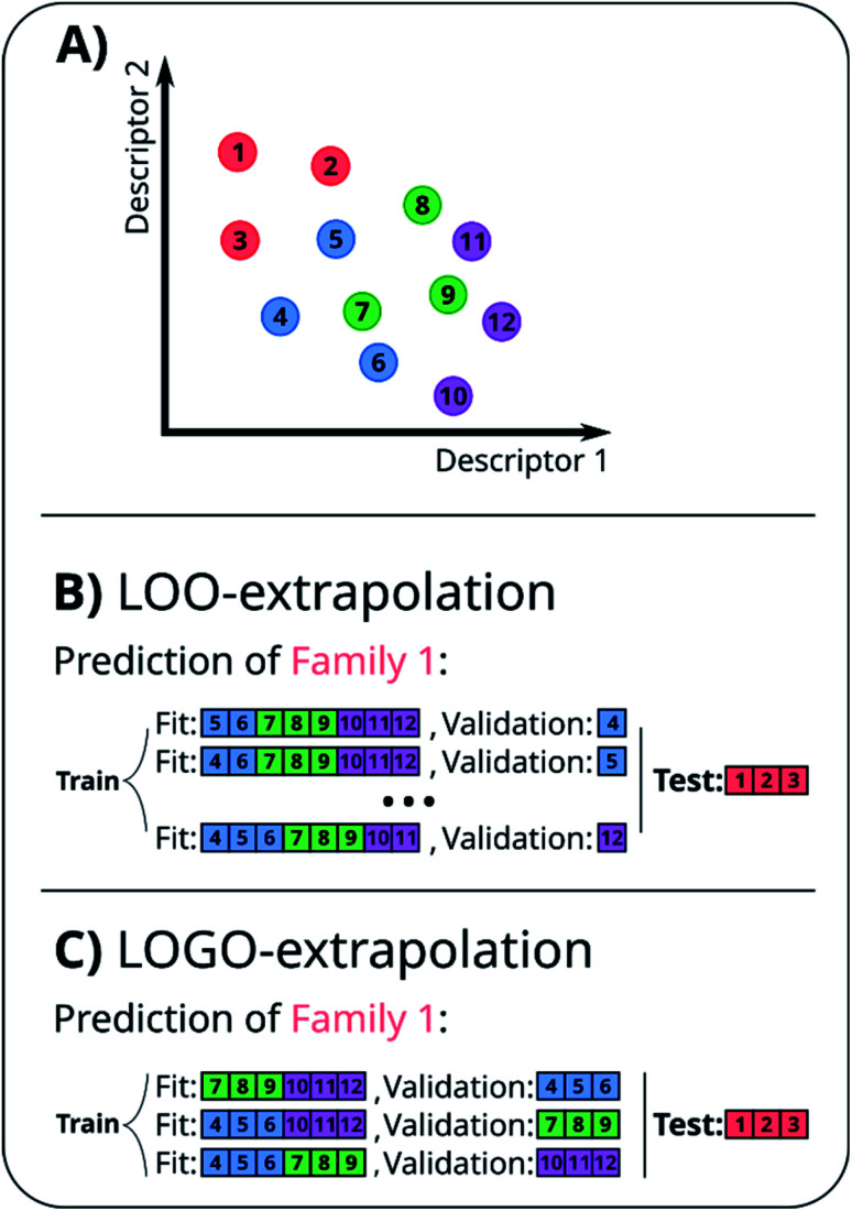
A naïve approach to deal with this issue would be to exclude all elements of a particular family A_n from the cross-validation, perform any form of cross-validation with the remaining data D − A_n and evaluate the predictive ability of the resulting method on the elements of A_n. This approach provides a measure of how well a standard ML approach predicts the properties of new families of compounds if no element of that family was used in its training. For example, one could perform a LOO cross-validation excluding in turn families of molecules, and we refer to this elementary approach as LOO-extrapolation. We show an example dataset with four distinct families in Fig. 2A, and we show in Fig. 2B how the data would be split with LOO-extrapolation to predict the values of one of these families. There have been similar approaches suggested recently, like the leave-one-cluster-out cross-validation,²⁹ where the dataset is split in clusters and one tries to predict the values for each cluster, which has been left out of the training set. Another approach is the k-fold-m-step forward cross-validation,³⁰ which ranks data by their target property value and evaluates how well the model can predict target values outside of the training domain, i.e. the model is trained to perform extrapolations of candidates in a different range of the target property, not necessarily to extrapolate to candidates from a different domain in the feature space. For example, a function tuned for prediction within the set D − A_n will be exploiting the existence of elements of the same family within D − A_n and it may not result in the best function to predict properties when no information on similar materials is available. The best chance to build a model able to perform accurate predictions on new families of materials is to train the model to do so.

Fig. 2. (A) Example of a small 2D database with 12 points split among four families, indicated by their color. (B) Representation of the LOO-extrapolation to predict the values of ‘Family 1’, where the algorithm is trained with a LOO cross-validation. (C) Representation of our proposed LOGO-extrapolation to predict the values of ‘Family 1’, where the algorithm is trained to extrapolate to other families and is finally tested to extrapolate the values of that new family.

We partition D in subgroups containing chemically distinct families {A_n}. For each subgroup A_m, we find the parameters h that minimize the following error:

3

In essence, leaving out group A_m, we consider in turn all the other groups A_n and compute the error in predicting elements in A_n without using the data in A_n (and neither A_m). The scheme is illustrated in Fig. 2C. Minimizing eqn (3) with respect to h is equivalent to finding the best function at performing extrapolations. This approach simulates a situation where no element of the family A_m has been discovered, and the remaining elements can be divided into distinct families. We call this method leave-one-group-out (LOGO) cross-validation. The procedure can be repeated for every A_m, where each one results in an optimal set of hyperparameters h^m,D_min,LOGO. The RMSE error can then be defined as:

4

We have referred to this use of a LOGO cross-validation to train the ML model to perform extrapolations as LOGO-extrapolation (see Fig. 2C). Note that this training can be applied to any ML algorithm, and it is ultimately based on a cross-validation approach that mimics the discovery of novel material classes to overcome the inherent ‘leakage’ of information that is present in other cross-validation methods. We are effectively optimizing the model's parameters so that they are good at generalizing predictions of novel groups. Similar goals to optimize the training process for a specific task can be found in the meta-learning of neural networks.^63,64

III. Chemical groups definition

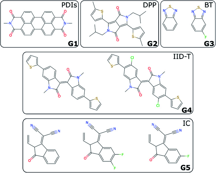
For non-fullerene acceptors, the grouping is based on the available literature with some additional considerations. Some recent reviews^25,65–68 have made attempts to classify the main acceptors by different chemical fragments such as perylene diimide (PDI),^65,67 isoindigo-based molecule (IID),⁶⁹ 1,8-naphthalimide (NI),⁷⁰ 2-(3-oxo-2,3-dihydroinden-1-ylidene (IC),⁷¹ diketopyrrolopyrrole (DPP),⁷² fluorene,⁷³ indacenodithiophene (IDT),^24,74 benzothiadiazole (BT),²⁴ benzodi(thienopyran) (BDTP),^75,76 (indacenodithieno[3,2-b]thiophene (IDTT),²⁴ terthieno[3,2-b]thiophene (6T)⁷⁷ and so forth. These conjugated fragments are responsible for the energy values of the acceptor's LUMO and donor's HOMO.⁷⁸ However, such classification does not immediately yield a partitioning of all non-fullerene acceptors into distinct non-overlapping groups. If the classification is too coarse-grained (e.g., molecules containing thiophenes), too many elements of different families will be grouped together; and if the classification is too fine-grained, there could be just one element in each group. We started by considering the type of fragments present in each acceptor (e.g., PDI, DPP, etc.). We show in Table S1† how we fingerprinted the 33 distinct acceptors in the database, by considering which of these fragments they contained. When it was ambiguous in which group to classify a particular acceptor, priority was given to the fragment where the LUMO – which gives the acceptor character – is localized. Any acceptor fragment containing more than 50% weight of the LUMO orbital density can be considered as a valid fragment, as shown in more detail in the ESI.† Note that this grouping process is relevant to the organic solar cells field, where groups of acceptor molecules with unique fragments have emerged over time, but specific knowledge of a field would be necessary to group data points into novel groups, as there is no unique standardized definition of novelty. At the end of this process, we have identified five groups of non-fullerene acceptors (G1-5): PDIs (with one or more monomers), DPP, BT, IID-T (IID unit connected with thiophene) and IC, which are illustrated in Fig. 3. In total, we classify 45 donor/acceptor pairs with non-fullerene acceptors in our five groups. Each of these groups contains between four and 25 donor/acceptor pairs from our database that broadly match the classification proposed in the literature.⁶⁹

Fig. 3. Illustration of investigated groups containing different fragments.

IV. LOO vs. LOGO

(a). LOGO extrapolation capabilities

In Table 1, we show the resulting RMSE in the ML prediction of several OPV molecules comparing a regular cross-validation (LOO) with a LOO-extrapolation and a LOGO extrapolation performed on the five groups identified in Fig. 3. When the extrapolation RMSE is much larger than the LOO RMSE, the ML method fails to describe the new family on the basis of existing knowledge. It has been studied before that fingerprints yield a similar or even better accuracy than physical descriptors when performing interpolation tasks.⁴⁶ However, this trend is reversed when trying to predict the PCE of new groups by training the model to extrapolate, where using physical descriptors is significantly better. This is an important point, as it shows that when one is trying to make predictions of molecules similar to those known by the model, one can rely solely on fingerprints to make accurate predictions, but one needs to use physical descriptors (and therefore a minimal understanding of the physics of the material) when predicting molecules from a new chemical family. Note that we are interested in describing extrapolations in structure space: predict the PCE of molecules that contain chemical groups and motifs unknown to the model. However, such an extrapolation does not necessarily mean an extrapolation of the physical descriptors, which are continuous.

RMSE (%) and Pearson correlation coefficient, r, results of PCE prediction using different cross-validation methods, with KRR. We have tried different features: fingerprints or physical descriptors.

	Features	RMSE (%)	r
LOO-interpolation	Fingerprints	1.75	0.69
	Physical descriptors	2.01	0.56
LOO-extrapolation	Fingerprints	3.52	0.08
	Physical descriptors	4.11	0.17
LOGO-extrapolation	Fingerprints	3.77	0.07
	Physical descriptors	2.84	0.31

A preliminary assessment of the data is offered by comparing the RMSE, as shown in Table 1. In this table, we can see how the correlation coefficient is very low and RMSE is large when using the fingerprints with either LOO-extrapolation or LOGO-extrapolation, indicating that extrapolating data based on this information alone is more challenging. We can also see how the LOGO extrapolation presents a clear improvement over the LOO-extrapolation. The best performance obtained with LOO-extrapolation results in a RMSE of 3.52%, and LOGO-extrapolation improves the RMSE to 2.84% (a relative improvement of 19%). Similarly, the best correlation obtained with LOGO-extrapolation (r = 0.31) is also significantly larger than the correlation obtained with LOO-extrapolation (0.08–0.17). To see this improvement when using LOGO-extrapolation, using a grouping with chemically distinct families, we present in Section S6.2 of the ESI† a comparison of LOO-extrapolation and LOGO-extrapolation when using another grouping. The best RMSE achieved with LOGO is still far from the one obtained with a regular LOO cross-validation (interpolating known data), and it results in a coefficient of determination of R² = 0.04, which makes it not suitable to perform quantitative predictions. However, researchers are not necessarily interested in a model that can make accurate quantitative predictions, and a model that can do a binary classification to separate candidate materials into well-performing and bad-performing can be equally helpful.

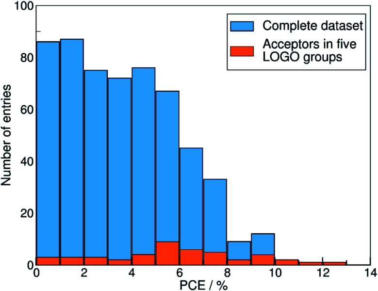
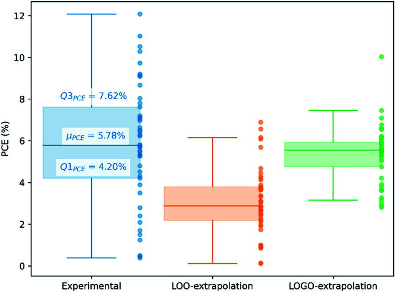
We show in Fig. 4 the PCE distribution of the complete dataset and the distribution for the 45 points corresponding to the non-fullerene materials classified into one of our five chemical groups, which we will try to predict. In Fig. 5, we show our PCE prediction of these 45 points when using LOO-extrapolation and LOGO-extrapolation, as well as the experimental PCE. One can clearly see how the LOGO-extrapolation distribution is much closer than the LOO-extrapolation one to the experimental PCE distribution (closer median and lower/upper quartile values), although both models struggle to predict high PCE values.

Fig. 4. Histogram with the PCE distribution of our complete dataset (in blue), and the PCE distribution of the 45 pairs with non-fullerene acceptors classified in the five groups used in the LOGO-extrapolation (in orange).

Fig. 5. PCE distribution of non-fullerene acceptors in our database, indicating the lower quartile (Q1_PCE), median (μ_PCE) and upper quartile (Q3_PCE). We also show the predicted PCE distributions with LOO-extrapolation and LOGO-extrapolation.

We have already mentioned the overall smaller RMSE and larger correlation (see Table 1) when adopting LOGO-extrapolation. However, we can go one step further and quantify how advantageous LOGO-extrapolation would be with respect to LOO-extrapolation when trying to identify materials over a certain threshold. We have used three different thresholds. We have chosen the lower quartile (Q1_PCE), median value (μ_PCE) and upper quartile (Q3_PCE) as statistically significant values to judge the ability of the model to do qualitative classifications (the threshold values are shown in Fig. 5). These thresholds allow to judge how the model performs for different classifications with an increasing difficulty:

(i) Identify materials with PCE > Q1_PCE. This simple threshold allows us to evaluate how well the model would do in identifying the worse performing materials.

(ii) Identify materials with PCE > μ_PCE. With this threshold, we have the best data distribution and we can classify candidate materials as well-performing and bad-performing, reducing possible candidates by half.

(iii) Identify materials with PCE > Q3_PCE. This threshold is more challenging, and allow us to quantify how many materials in the top 25% of our dataset are correctly predicted within that range.

Each predicted PCE can be classified as true positive (TP), false positive (FP), true negative (TN) or false negative (FN), as shown in Table 2.

Confusion matrix when classifying PCE above a threshold.

	Predicted PCE > threshold	Predicted PCE < threshold
Actual PCE > threshold	True positive (TP)	False negative (FN)
Actual PCE < threshold	False positive (FP)	True negative (TN)

We can directly measure the accuracy of our model by calculating the probability of making a correct prediction:

5

Additionally, we also calculate the precision, P, as the fraction of predicted well-performing materials that are actually well-performing,

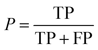6

and the recall, R, as the fraction of actual well-performing materials that are predicted to be well-performing

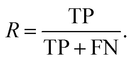7

These metrics are common for these types of binary classifications,^79,80 and they are often averaged in a single metric, the F₁-score, which we use as another indicator of the classification accuracy:

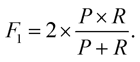8

We show the results for the two thresholds PCE > Q1_PCE and PCE > μ_PCE in Table 3. For the lowest threshold of PCE > Q1_PCE, it is worth noting how a LOO-extrapolation results in a mediocre accuracy and F₁-score (A = 0.33 and F₁ = 0.29). The precision is relatively high (P = 0.67), but the recall is quite low (R = 0.18), which means that we are missing most of the actual well-performing materials. However, when we use a LOGO cross-validation, both the accuracy and F₁-score are significantly larger (A = 0.80 and F₁ = 0.87), and the number of false negatives is reduced further, resulting in a larger recall (R = 0.88). In other words, if no special care is taken, an ML algorithm trained with a regular cross-validation performs very poorly when trying to predict new classes of molecules. However, a suitable cross-validation, like the one proposed in the LOGO-extrapolation, can significantly improve the predictive power of the ML model. When we use a higher threshold, PCE > μ_PCE, we observe a similar trend, although now both LOO-extrapolation and LOGO-extrapolation result in the same accuracy (A = 0.51) and a similar precision (P = 0.50 and P = 0.53, respectively). However, LOGO-extrapolation still results in a much larger recall and F₁-score (R = 0.35 and F₁ = 0.42) when compared to LOO-extrapolation (R = 0.09 and F₁ = 0.15). When we use the most challenging threshold of PCE > Q3_PCE, both LOO-extrapolation and LOGO-extrapolation struggle and they are not able to correctly predict any of the points in that interval. Therefore, it seems that this approach is advantageous to identify low-performing materials, but is unable to correctly identify high-performing materials. We show in Fig. S2 in the ESI† all real and predicted values when using LOO-extrapolation and LOGO-extrapolation.

Metrics obtained with a LOO-extrapolation and LOGO-extrapolation, with KRR, when classifying materials with PCE > Q1_PCE and PCE > μ_PCE.

Metric	PCE > Q1PCE		PCE > μPCE
	LOO-extrapolation	LOGO-extrapolation	LOO-extrapolation	LOGO-extrapolation
TP	6	30	2	8
FP	3	5	2	7
TN	9	6	21	15
FN	27	4	20	15
Accuracy	0.33	0.80	0.51	0.51
Precision	0.67	0.86	0.50	0.53
Recall	0.18	0.88	0.09	0.35
F 1-Score	0.29	0.87	0.15	0.42

(b). LOGO convergence to LOO

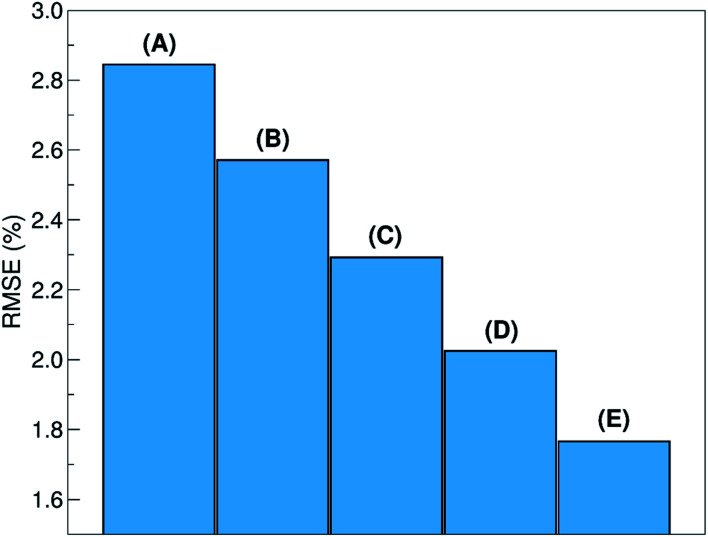
The relative ability to predict completely new chemistries is intuitively related to the novelty of the molecules to be considered, with respect to the training set. To better understand the relation between the proposed LOGO-extrapolation and the conventional LOO-interpolation, it is instructive to see how the prediction RMSE is affected by changing the definition of groups, which we exemplify in Fig. 6 through the use of five models. The prediction RMSE is the largest when we classify the donor/acceptor pairs with non-fullerene acceptors in the five groups defined on the basis of chemical similarity, as in Section III (model A). The RMSE improves as the pairs with non-fullerene acceptor molecules are grouped in five random groups (model B). The RMSE is reduced further when we consider all donor/acceptor pairs, where each group contains just the pairs with one of the 33 acceptor molecules (model C), and even more if we increase the number of groups to 55 (model D), where some acceptor molecules are present in more than one group. The best RMSE value is found when the LOO cross-validation is used (model E). This progression of cases exemplifies the gradual change from a model performing pure extrapolation (less accurate but more useful) toward a model performing pure interpolation (more accurate but less useful). We show in the ESI† more details on how these groups were selected.

Fig. 6. Prediction RMSE, using LOGO-extrapolation with different groups: (A) non-fullerene acceptors split in five chemically distinct families; (B) non-fullerene acceptors split in five random groups; (C) all acceptors split in 33 random groups; (D) all acceptors split in 55 random groups. (E) Prediction RMSE using LOO-interpolation.

V. Example of model deployment

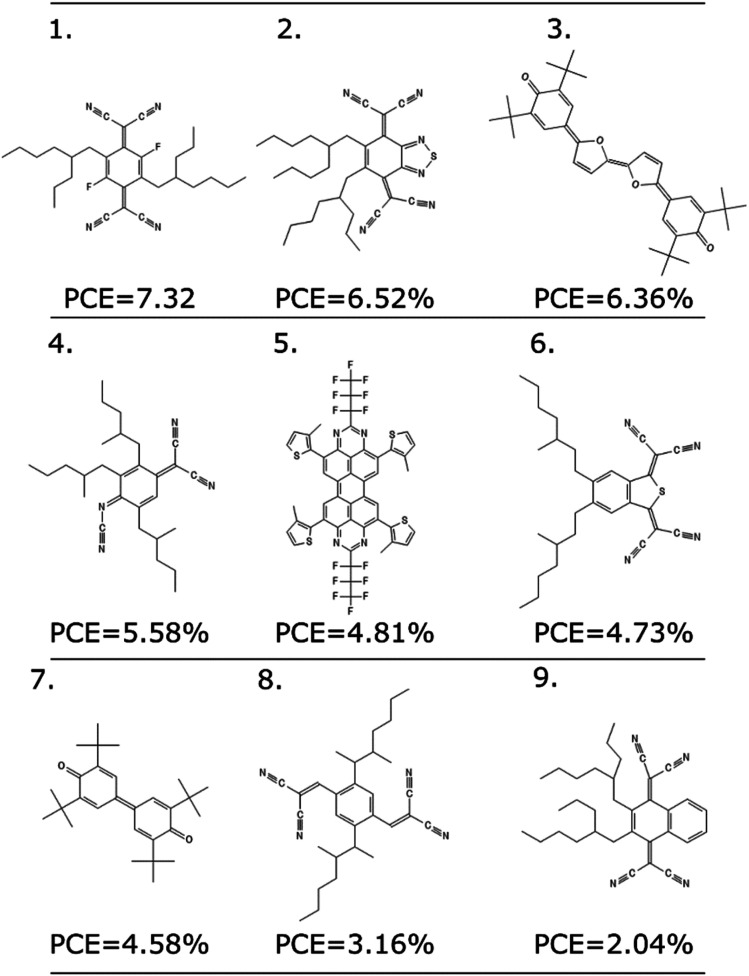
As any other ML methodology, this approach can be used to evaluate the efficiency of molecules not present in the data set, which can be obtained from experimental intuition, a database search or a more complicated generative model.²³ To illustrate the possible applications, we identified nine molecules from a database of computed electronic properties of known molecules developed in ref. 81. We considered molecules with physical descriptors in the same range of high performing non-fullerene acceptors: LUMO energy lower than −2.85 eV and ∑f larger than 0.8, and we have added alkyl side chains to match more closely the solubility parameter of the best performing examples. See Section S7 of the ESI† for more details of how these molecules were selected and the optimized hyperparameters of the model.

We excluded molecules that belonged to any of the known classes of non-fullerene acceptors in our dataset. Fig. 7 reports nine molecules, along with their predicted PCE, when combined with the best performing donor in our database (ZnP-TBO⁸²). We can see how the PCE range of these molecules is similar to the range predicted for the other non-fullerene acceptor groups (see Fig. 5), and three of them have a predicted PCE above the median value for all other NFA in the database, which suggests them as high interest candidates. Additional considerations like cost and ease of synthesis from precursor could be considered, and domain knowledge would be particularly critical in the design phase.

Fig. 7. Nine molecules unknown to the model, and their suggested PCE using the LOGO-extrapolation framework, with KRR and physical descriptors.

VI. Conclusions

In summary, we proposed a training method to improve the extrapolation capabilities of ML models to materials from completely new families, and we applied it to the prediction of the performance of non-fullerene acceptors. Our results show that the quantitative prediction error in these extrapolative tasks is larger than the one achieved by predicting molecules within known chemical families. To address this shortcoming, we propose a method based on a leave-one-group-out (LOGO) cross-validation, in which we train an ML model to accurately perform extrapolations on unseen families of compounds. We have shown this choice results in an RMSE improvement and a significant success rate in classifying unseen materials above and below the median efficiency, when compared to a method trained with an ordinary cross-validation. We have observed that when extrapolating to new chemical families, physical descriptors are needed to make accurate predictions, and cheap fingerprints are not enough, unlike when one is predicting molecules within known chemical families. Finally, we have seen how the LOGO cross-validation accuracy converges towards the accuracy obtained with a regular cross-validation when one ignores the existence of chemical families. These results are promising and suggest that, in fields where data becomes structured into recognizable families, using training methods like the proposed LOGO cross-validation can accelerate the discovery of completely new families.

Data availability

The dataset used during the current study, as well as the code used to perform the analysis and scripts to reproduce the main results are available in a public GitHub repository at www.github.com/marcosdelcueto/NonFullereneAcceptorPrediction.

Author contributions

A. T. designed the project. M. d. C and A. T. developed the theoretical formalism. Z.-W. Z. created the database. M. d. C. performed the ML analysis. All authors contributed to the analysis of the results and writing of the manuscript.

Conflicts of interest

There are no conflicts to declare.

References

- Gromski P. S. Henson A. B. Granda J. M. Cronin L. Nat. Rev. Chem. 2019;3:119–128. doi: 10.1038/s41570-018-0066-y. [DOI] [Google Scholar]
- Awale M. Visini R. Probst D. Arus-Pous J. Reymond J. L. Chimia. 2017;71:661–666. doi: 10.2533/chimia.2017.661. [DOI] [PubMed] [Google Scholar]
- Coley C. W. Eyke N. S. Jensen J. F. Angew. Chem., Int. Ed. 2019;59:23414–23436. doi: 10.1002/anie.201909989. [DOI] [PubMed] [Google Scholar]
- Mahmood A. Wang J.-L. Energy Environ. Sci. 2021;14:90–105. doi: 10.1039/D0EE02838J. [DOI] [Google Scholar]
- Oliynyk A. O. Buriak J. M. Chem. Mater. 2019;31:8243–8247. doi: 10.1021/acs.chemmater.9b03854. [DOI] [Google Scholar]
- Chen C. Zuo Y. Ye W. Li X. Deng Z. Ong S. P. Adv. Energy Mater. 2020;10:1903242. doi: 10.1002/aenm.201903242. [DOI] [Google Scholar]
- Schmidt J. Marques M. R. G. Botti S. Marques M. A. L. npj Comput. Mater. 2019;5:83. doi: 10.1038/s41524-019-0221-0. [DOI] [Google Scholar]
- Rodríguez-Martínez X. Pascual-San-José E. Campoy-Quiles M. Energy Environ. Sci. 2021;14:3301–3322. doi: 10.1039/D1EE00559F. [DOI] [PMC free article] [PubMed] [Google Scholar]
- Liu Y. Esan O. C. Pan Z. An L. Energy and AI. 2021;3:100049. doi: 10.1016/j.egyai.2021.100049. [DOI] [Google Scholar]
- Zhou Z. Zhou Y. He Q. Ding Z. Li F. Yang Y. npj Comput. Mater. 2019;5:128. doi: 10.1038/s41524-019-0265-1. [DOI] [Google Scholar]
- Wu S. Kondo Y. Kakimoto M. Yang B. Tamada H. Kuwajima I. Lambard G. Hongo K. Xu Y. Shiomi J. Schick C. Morikawa J. Yoshida R. npj Comput. Mater. 2019;5:66. doi: 10.1038/s41524-019-0203-2. [DOI] [Google Scholar]
- Balachandran P. V. Kowalski B. Sehirlioglu A. Lookman T. Nat. Commun. 2018;9:1668. doi: 10.1038/s41467-018-03821-9. [DOI] [PMC free article] [PubMed] [Google Scholar]
- Fischer C. C. Tibbetts K. J. Morgan D. Ceder G. Nat. Mater. 2006;5:641–646. doi: 10.1038/nmat1691. [DOI] [PubMed] [Google Scholar]
- Hautier G. Fischer C. C. Jain A. Mueller T. Ceder G. Chem. Mater. 2010;22:3762–3767. doi: 10.1021/cm100795d. [DOI] [Google Scholar]
- Hautier G. Fischer C. Ehrlacher V. Jain A. Ceder G. Inorg. Chem. 2011;50:656–663. doi: 10.1021/ic102031h. [DOI] [PubMed] [Google Scholar]
- Dey P. Bible J. Datta D. Broderick S. Jasinski J. Sunkara M. Menon M. Rajan K. Comput. Mater. Sci. 2014;83:185–195. doi: 10.1016/j.commatsci.2013.10.016. [DOI] [Google Scholar]
- Oliynyk A. O. Adutwum L. A. Harynuk J. J. Mar A. Chem. Mater. 2016;28:6672–6681. doi: 10.1021/acs.chemmater.6b02905. [DOI] [Google Scholar]
- Ryan K. Lengyel J. Shatruk M. J. Am. Chem. Soc. 2018;140:10158–10168. doi: 10.1021/jacs.8b03913. [DOI] [PubMed] [Google Scholar]
- Kailkhura B. Gallagher B. Kim S. Hiszpanski A. Han T. Y.-J. npj Comput. Mater. 2019;5:108. doi: 10.1038/s41524-019-0248-2. [DOI] [Google Scholar]
- Mitchell J. B. O. Wiley Interdiscip. Rev.: Comput. Mol. Sci. 2014;4:468–481. doi: 10.1002/wcms.1183. [DOI] [PMC free article] [PubMed] [Google Scholar]
- Krstajic D. Buturovic L. J. Leahy D. E. Thomas S. J. Cheminf. 2014;6:10. doi: 10.1186/1758-2946-6-10. [DOI] [PMC free article] [PubMed] [Google Scholar]
- Sahu H. Rao W. Troisi A. Ma. H. Adv. Energy Mater. 2018;8:1801032. doi: 10.1002/aenm.201801032. [DOI] [Google Scholar]
- Peng S.-P. Zhao Y. J. Chem. Inf. Model. 2019;59:4993–5001. doi: 10.1021/acs.jcim.9b00732. [DOI] [PubMed] [Google Scholar]
- Wadsworth A. Moser M. Marks A. Little M. S. Gasparini N. Brabec C. J. Baran D. McCulloch I. Chem. Soc. Rev. 2019;48:1596–1625. doi: 10.1039/C7CS00892A. [DOI] [PubMed] [Google Scholar]
- Hou J. Inganäs O. Friend R. H. Gao F. Nat. Mater. 2018;17:119–128. doi: 10.1038/nmat5063. [DOI] [PubMed] [Google Scholar]
- Yan C. Barlow S. Wang Z. Yan H. Jen A. K.-Y. Marder S. R. Zhan X. Nat. Rev. Mater. 2018;3:18003. doi: 10.1038/natrevmats.2018.3. [DOI] [Google Scholar]
- Lin Y. Wang J. Zhang Z.-G. Bai H. Li Y. Zhu D. Zhan X. Adv. Mater. 2015;27:1170–1174. doi: 10.1002/adma.201404317. [DOI] [PubMed] [Google Scholar]
- Cui Y. Yao H. Zhang J. Xian K. Zhang T. Hong L. Wang Y. Xu Y. Ma K. An C. He C. Wei Z. Gao G. Hou J. Adv. Mater. 2020;32:1908205. doi: 10.1002/adma.201908205. [DOI] [PubMed] [Google Scholar]
- Meredig B. Antono E. Church C. Hutchinson M. Ling J. Paradiso S. Blaiszik B. Foster I. Gibbons B. Hattrick-Simpers J. Mehta A. Ward L. Mol. Syst. Des. Eng. 2018;3:819–825. doi: 10.1039/C8ME00012C. [DOI] [Google Scholar]
- Xiong Z. Cui Y. Liu Z. Zhao Y. Hu M. Hu J. Comput. Mater. Sci. 2020;171:109203. doi: 10.1016/j.commatsci.2019.109203. [DOI] [Google Scholar]
- Ahneman D. T. Estrada J. G. Lin S. Dreher S. D. Doyle A. G. Science. 2018;360:6385. doi: 10.1126/science.aar5169. [DOI] [PubMed] [Google Scholar]
- Estrada J. G. Ahneman D. T. Sheridan R. P. Dreher S. D. Doyle A. G. Science. 2018;362:6416. doi: 10.1126/science.aat8763. [DOI] [PubMed] [Google Scholar]
- Jin W., Barzilay R. and Jaakkola T., arXiv:2006,03908, 2020
- Cheng P. Li G. Zhan X. Yang Y. Nat. Photonics. 2018;12:131–142. doi: 10.1038/s41566-018-0104-9. [DOI] [Google Scholar]
- Sahu H. Yang F. Ye X. Ma J. Fang W. Ma H. J. Mater. Chem. A. 2019;7:17480–17488. doi: 10.1039/C9TA04097H. [DOI] [Google Scholar]
- Lopez S. A. Pyzer-Knapp E. O. Simm G. N. Lutzow T. Li K. Seress L. R. Hachmann J. Aspuru-Guzik A. Sci. Data. 2016;3:160086. doi: 10.1038/sdata.2016.86. [DOI] [PMC free article] [PubMed] [Google Scholar]
- Paul A. Furmanchuk A. Liao W. K. Choudhary A. Agrawal A. Mol. Inf. 2019;38:e1900038. doi: 10.1002/minf.201900038. [DOI] [PubMed] [Google Scholar]
- Meftahi N. Klymenko M. Christofferson A. J. Bach U. Winkler D. A. Russo S. P. npj Comput. Mater. 2020;6:166. doi: 10.1038/s41524-020-00429-w. [DOI] [Google Scholar]
- Wu Y. Guo J. Sun R. Min J. npj Comput. Mater. 2020;6:120. doi: 10.1038/s41524-020-00388-2. [DOI] [Google Scholar]
- Li J. Pradhan B. Gaur S. Thomas J. Adv. Energy Mater. 2019;9:1901891. doi: 10.1002/aenm.201901891. [DOI] [Google Scholar]
- David T. W. Anizelli H. Jacobsson T. J. Gray C. Teahan W. Kettle J. Nano Energy. 2020;78:105342. doi: 10.1016/j.nanoen.2020.105342. [DOI] [Google Scholar]
- Krawczyk B. Prog. Artif. Intell. 2016;5:221–232. doi: 10.1007/s13748-016-0094-0. [DOI] [Google Scholar]
- Raccuglia P. Elbert K. C. Adler P. D. F. Falk C. Wenny M. B. Mollo A. Zeller M. Friedler S. A. Schrier J. Norquist A. J. Nature. 2016;533:73–76. doi: 10.1038/nature17439. [DOI] [PubMed] [Google Scholar]
- Cao B. Adutwum L. A. Oliynyk A. O. Luber E. J. Olsen B. C. Mar A. M Buriak J. ACS Nano. 2018;12:7434–7444. doi: 10.1021/acsnano.8b04726. [DOI] [PubMed] [Google Scholar]
- del Cueto M. Troisi A. Phys. Chem. Chem. Phys. 2021;23:14156–14163. doi: 10.1039/D1CP01761F. [DOI] [PubMed] [Google Scholar]
- Zhao Z.-W. del Cueto M. Geng Y. Troisi A. Chem. Mater. 2020;32:7777–7787. doi: 10.1021/acs.chemmater.0c02325. [DOI] [Google Scholar]
- del Cueto M., Non-Fullerene Acceptor Prediction, github.com/marcosdelcueto/NonFullereneAcceptorPrediction, 2022
- Padula D. Troisi A. Adv. Energy Mater. 2019;9:1902463. doi: 10.1002/aenm.201902463. [DOI] [Google Scholar]
- Rogers D. Hahn M. J. Chem. Inf. Model. 2010;50:742–754. doi: 10.1021/ci100050t. [DOI] [PubMed] [Google Scholar]
- Schober C. Reuter K. Oberhofer H. J. Phys. Chem. Lett. 2016;7:3973–3977. doi: 10.1021/acs.jpclett.6b01657. [DOI] [PubMed] [Google Scholar]
- Lopez S. A. Sanchez-Lengeling B. Soares J. G. Aspuru-Guzik A. Joule. 2017;1:857. doi: 10.1016/j.joule.2017.10.006. [DOI] [Google Scholar]
- Cheng T. Zhao Y. Li X. Lin F. Xu Y. Zhang X. Li Y. Wang R. Lai L. J. Chem. Inf. Model. 2007;47:2140–2148. doi: 10.1021/ci700257y. [DOI] [PubMed] [Google Scholar]
- Mannhold R. Poda G. I. Ostermann C. Tetko I. V. J. Pharm. Sci. 2009;98:861–893. doi: 10.1002/jps.21494. [DOI] [PubMed] [Google Scholar]
- Daina A. Michielin O. Zoete V. Sci. Rep. 2017;7:42717. doi: 10.1038/srep42717. [DOI] [PMC free article] [PubMed] [Google Scholar]
- Padula D. Simpson J. D. Troisi A. Mater. Horiz. 2019;6:343–349. doi: 10.1039/C8MH01135D. [DOI] [Google Scholar]
- Jung H. Stocker S. Kunkel C. Oberhofer H. Han B. Reuter K. Margraf J. T. ChemSystemsChem. 2020;2:e1900052. doi: 10.1002/syst.201900052. [DOI] [Google Scholar]
- Altman N. S. Am. Stat. 1992;46:175–185. [Google Scholar]
- Smola A. J. Schölkopf B. A. Stat. Comput. 2004;14:199–222. doi: 10.1023/B:STCO.0000035301.49549.88. [DOI] [Google Scholar]
- Bajusz D. Racz A. Heberger K. J. Cheminf. 2015;7:1–13. doi: 10.1186/s13321-015-0069-3. [DOI] [PMC free article] [PubMed] [Google Scholar]
- Storn R. Price K. J. Glob. Optim. 1997;11:341–359. doi: 10.1023/A:1008202821328. [DOI] [Google Scholar]
- Virtanen P. et al. . Nat. Methods. 2020;17:261–272. doi: 10.1038/s41592-019-0686-2. [DOI] [PMC free article] [PubMed] [Google Scholar]
- Finn C., Abbeel P. and Levine S., Proceedings of the 38th International Conference on Machine Learning, 2017, vol. 70, pp. 1126–1135 [Google Scholar]
- Bai Y., Chen M., Zhou P., Zhao T., Lee J., Kakade S., Wang H. and Xiong C., Proceedings of the 38th International Conference on Machine Learning, 2021, vol. 139, pp. 543–553 [Google Scholar]
- Zhang G. Zheo J. Chow P. C. Y. Jiang K. Zhang J. Zhu Z. Zhang J. Huang F. Yan H. Chem. Rev. 2018;118:3447–3507. doi: 10.1021/acs.chemrev.7b00535. [DOI] [PubMed] [Google Scholar]
- Zhang J. Tan H. S. Guo X. Facchetti A. Yan H. Nat. Energy. 2018;3:720–731. doi: 10.1038/s41560-018-0181-5. [DOI] [Google Scholar]
- Nielsen C. B. Holliday S. Chen H. Y. Cryer S. J. McCulloch I. Acc. Chem. Res. 2015;48:2803–2812. doi: 10.1021/acs.accounts.5b00199. [DOI] [PMC free article] [PubMed] [Google Scholar]
- Li S. Liu W. Li C.-Z. Shi M. Chen H. Small. 2017;13:1701120. doi: 10.1002/smll.201701120. [DOI] [PubMed] [Google Scholar]
- Zhang B. An N. Wu H. Geng Y. Sun Y. Ma Z. Li W. Guo Q. Zhou E. Sci. China: Chem. 2020;63:1262–1271. doi: 10.1007/s11426-020-9777-1. [DOI] [Google Scholar]
- Zhang J. Zhang X. Xiao H. Li G. Liu Y. Li C. Huang H. Chen X. Bo Z. ACS Appl. Mater. Interfaces. 2016;8:5475–5483. doi: 10.1021/acsami.5b10211. [DOI] [PubMed] [Google Scholar]
- Suman Singh S. P. J. Mater. Chem. A. 2019;7:22701–22729. doi: 10.1039/C9TA08620J. [DOI] [Google Scholar]
- Bijleveld J. C. Gevaerts V. S. Di Nuzzo D. Turbiez M. Mathijssen S. G. J. de Leeuw D. Wienk M. M. Janssen R. A. J. Adv. Mater. 2010;22:E242–E246. doi: 10.1002/adma.201001449. [DOI] [PubMed] [Google Scholar]
- Suman Bagui A. Datt R. Gupta V. Singh S. P. Chem. Commun. 2017;53:12790–12793. doi: 10.1039/C7CC08237A. [DOI] [PubMed] [Google Scholar]
- Wu F. Zhong L. Hiu H. Li Y. Zhang Z. Li Y. Zhang Z.-G. Ade H. Jiang Z.-Q. Liao L.-S. J. Mater. Chem. A. 2019;7:4063–4071. doi: 10.1039/C8TA11972D. [DOI] [Google Scholar]
- Wu H. Fan H. Xu S. Zhang C. Chen S. Yang C. Chen D. Liu F. Zhu X. Sol. RRL. 2017;1:1700165. doi: 10.1002/solr.201700165. [DOI] [Google Scholar]
- Wu H. Fan H. Xu S. Ye L. Guo Y. Yi Y. Ade H. Zhu X. Small. 2019;15:1804271. doi: 10.1002/smll.201804271. [DOI] [PubMed] [Google Scholar]
- Shi X. Chen J. Gao K. Zuo L. Yao Z. Liu F. Tang J. Jen A. K.-Y. Adv. Energy Mater. 2018;8:1702831. doi: 10.1002/aenm.201702831. [DOI] [Google Scholar]
- Kuzmich A. Padula D. Ma H. Troisi A. Energy Environ. Sci. 2017;10:395–401. doi: 10.1039/C6EE03654F. [DOI] [Google Scholar]
- Li W. Jacobs R. Morgan D. Comput. Mater. Sci. 2018;150:454–463. doi: 10.1016/j.commatsci.2018.04.033. [DOI] [Google Scholar]
- Weston L. Stampfl C. Phys. Rev. Mater. 2018;2:085407. doi: 10.1103/PhysRevMaterials.2.085407. [DOI] [Google Scholar]
- Padula D. Omar O. H. Nematiaram T. Troisi A. Energy Environ. Sci. 2019;12:2412–2416. doi: 10.1039/C9EE01508F. [DOI] [Google Scholar]
- Gao K. Jo S. B. Shi X. Nian L. Zhang M. Kan Y. Lin F. Kan B. Xu B. Rong Q. Shui L. Liu F. Peng X. Zhou G. Cao Y. Jen A. K.-Y. Adv. Mater. 2019;31:1807842. doi: 10.1002/adma.201807842. [DOI] [PubMed] [Google Scholar]
Associated Data
This section collects any data citations, data availability statements, or supplementary materials included in this article.
Supplementary Materials
Data Availability Statement