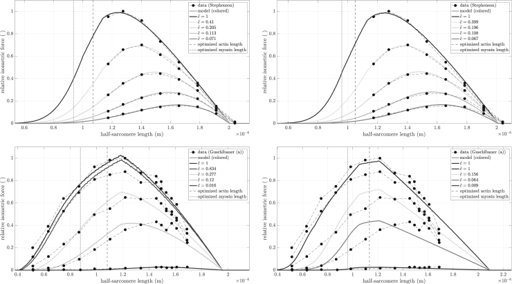
Figure B. 13.
Best (Stephenson, upper row) and worst (Guschlbauer (a), lower row) examples of fixing non-sensitive parameters. Left column shows results from the parameter fit with bounds from Table 4. Right column shows the optimal fit after fixing the nine most insensitive parameters. Note that for Guschlbauer (a), the fits to the two highest activation FLAR datasets were identical (both found ). For residuals, see Table B1. To see this figure in color, go online.

