

Abstract
In this paper, a new stochastic optimization algorithm is introduced, called Driving Training-Based Optimization (DTBO), which mimics the human activity of driving training. The fundamental inspiration behind the DTBO design is the learning process to drive in the driving school and the training of the driving instructor. DTBO is mathematically modeled in three phases: (1) training by the driving instructor, (2) patterning of students from instructor skills, and (3) practice. The performance of DTBO in optimization is evaluated on a set of 53 standard objective functions of unimodal, high-dimensional multimodal, fixed-dimensional multimodal, and IEEE CEC2017 test functions types. The optimization results show that DTBO has been able to provide appropriate solutions to optimization problems by maintaining a proper balance between exploration and exploitation. The performance quality of DTBO is compared with the results of 11 well-known algorithms. The simulation results show that DTBO performs better compared to 11 competitor algorithms and is more efficient in optimization applications.
Subject terms: Engineering, Mathematics and computing
Introduction
Optimization is the process that determines the best solution to a problem with several feasible solutions. An optimization problem consists of three parts: decision variables, constraints, and the objective function1. In this case, the purpose of optimization is to quantify the decision variables with respect to the constraints of the problem so that the value of the objective function is optimized2. With the advancement of science and technology, the importance and role of optimization in various branches of science have become clearer. Therefore, practical tools are needed to address the various optimization challenges. Optimization techniques fall into two groups: deterministic and stochastic approaches. Deterministic approaches in both gradient-based and nongradient-based groups are effective in linear, convex, uncomplicated, low-dimensional, and differentiable problems. However, these approaches lose their effectiveness in dealing with optimization problems that have features such as nonlinear, nonconvex, complex, high-dimensional, notdifferentiable, discrete search space, and NP-hard problems. The difficulties and inefficiencies of deterministic approaches have led to the emergence of stochastic approaches that, using random operators, random search, and trial-and-error processes, are effective in optimization applications. Metaheuristic optimization algorithms, known as stochastic approaches, have become very popular and widely used due to advantages such as simple concepts, easy implementation, independent of the type of problem, no need for objective function-derived information, and efficiency in nonlinear, nonconvex environments, and nonlinear search space3. The optimization process in metaheuristic algorithms starts with generating a number of random candidate solutions in the range allowed for the search space. Then, in an iterative process, the candidate solutions are improved by the algorithm steps. After completion of the algorithm implementation iterations, the best candidate solution is introduced as the solution to the problem. The nature of random search in metaheuristic algorithms leads to the fact that there is no guarantee that this best candidate solution is the best solution (known as the global optimal) to a problem. Therefore, the best candidate solution is known as a quasi-optimal solution, which is an acceptable solution and close to the global optimal4. Achieving better quasi-optimal solutions has become a challenge in optimization studies to motivate researchers to introduce and design countless metaheuristic algorithms. In designing optimization algorithms, two indicators of exploration and exploitation play an important role in the performance of optimization algorithms in achieving appropriate quasi-optimal solutions. Exploring indicates the ability of the algorithm to perform a global search, and exploitation indicates the ability of the algorithm to perform a local search in the search space. The key to the success of a metaheuristic algorithm in the optimization process is maintaining a suitable balance between exploration and exploitation5. The main research question is whether, given that numerous optimization algorithms have been developed so far, is there still a need to design newer algorithms? The answer to this question, given the concept of No Free Lunch (NFL)6, is that there is no guarantee that an algorithm will work the same in all optimization problems. The NFL states that an algorithm may have a successful implementation on some optimization issues but fail to address others. Consequently, a particular algorithm cannot be considered the best optimizer for all optimization problems. Influenced by the concept of the NFL theorem, authors are encouraged to come up with more effective solutions to optimization problems by introducing new optimizers. The NFL theorem also motivated the authors of this paper to develop a new metaheuristic algorithm to address optimization applications. The novelty and contribution of this paper are in the design of a new metaheuristic algorithm called Driving Training-Based Optimization (DTBO), which is based on the simulation of human activity in driving education. The contributions of this paper are as follows:
DTBO is introduced based on the driving training process in which a person is trained to learn driving skills.
A set of 53 objective functions is used to analyze the performance of DTBO in optimization applications.
To evaluate the quality of the performance of DTBO, the results obtained are compared with the results of 11 well-known optimization algorithms.
The efficiency of DTBO is evaluated in solving two real-world applications.
The rest of the article is organized in such a way that in the “Lecture review”, the literature review is presented. In “Driving training based optimization”, the proposed DTBO approach is introduced and modeled. In “Computational complexity of DTBO”, simulation studies and results are presented. A discussion of the results and performance of the DTBO is provided in “Discussion. The application of DTBO in solving real-world problems is evaluated in the “DTBO for real-world applications”. The conclusions and several perspectives of the study are provided in “Conclusion and future works” section.
Lecture review
Meta-heuristic algorithms have been developed inspired by various natural phenomena, wildlife, animals, birds, insects, plants, living organisms, laws of physics, biological sciences, genetics, rules of games, human activities, and other natural evolutionary processes. In a grouping based on the design’s primary inspiration, metaheuristic algorithms fall into five groups: swarm-based, evolutionary-based, physics-based, game-based, and human-based methods.
Swarm-based metaheuristic algorithms have been developed to model the swarming behaviors of animals, birds, and living things in nature. Among the famous algorithms that can be mentioned are Particle Swarm Optimization (PSO)7, Firefly Algorithm (FA)8, Artificial Bee Colony (ABC)9, and Ant Colony Optimization (ACO)10. The natural behavior of a group of birds or fish in search of food, while their movement is influenced by personal experience and swarming intelligence, has been the main idea in PSO design. Mathematical modeling of the natural feature of flashing lights in fireflies has been used in the FA design. The primary inspiration in ABC design is to simulate the intelligence of swarming bee colonies to find food sources. The ability of an ant colony to find the shortest path between the colony and food sources has been the main idea in the design of the ACO. Hunting and attacking prey strategy, as well as the process of finding food sources among living organisms, has been a source of inspiration in designing various metaheuristic algorithms such as the Tunicate Search Algorithm (TSA)11, Reptile Search Algorithm (RSA)12, Whale Optimization Algorithm (WOA)13, Orca Predation Algorithm (OPA)14, Marine Predator Algorithm (MPA)15, Pelican Optimization Algorithm (POA)16, Snow Leopard Optimization Algorithm (SLOA)17, Gray Wolf Optimization (GWO) algorithm18, Artificial Gorilla Troops Optimizer (GTO)19, African Vultures Optimization Algorithm (AVOA)20, Farmland Fertility21, Spotted Hyena Optimizer (SHO)22, and Tree Seed Algorithm (TSA)23.
Evolutionary-based metaheuristic algorithms have been introduced based on simulations of biological sciences, genetics, and using random operators. Among the most widely used and well-known evolutionary algorithms, you can name the Genetic Algorithm (GA)24 and Differential Evolutionary (DE)25. GA and DE have been developed on the basis of mathematical modeling of the reproductive process and the concept of natural selection, as well as the employment of random operators of selection, crossover, and mutation.
Physics-based metaheuristic algorithms are designed on the basis of mathematical modeling of various physical laws and phenomena. Among the well-known physics-based algorithms, one can mention the Simulated Annealing (SA)26 and the Gravitational Search Algorithm (GSA)27. SA is based on the physical phenomenon of melting and then cooling metals, known in metallurgy as annealing. The modeling of Gravitational Forces in a system consisting of objects with different masses and distances from each other has been the main inspiration in the design of GSAs. The physical phenomenon of the water cycle and its transformations in nature has been a source of inspiration for the design of the Water Cycle Algorithm (WCA)28. Cosmological concepts have been the main inspiration in the design of the Multi-Verse Optimizer (MVO)29. Some other physics-based methods are as follows: Flow Regime Algorithm (FRA)30, Nuclear Reaction Optimization (NRO)31, Spring Search Algorithm (SSA)32, and Equilibrium Optimizer (EO)33.
Game-based metaheuristic algorithms have been developed based on simulation of the rules that govern different games and the behavior of players, coaches, and other individuals who influence the games. The design of modeling competitions in the volleyball league has been the main idea in the design of the Volleyball Premier League (VPL) algorithm34 and the football league has been the main idea in the design of Football Game-Based Optimization (FGBO)35. The strategy and skill of the players to create puzzle pieces has been the main inspiration in designing the Puzzle Optimization Algorithm (POA)36. The effort of the players in tug-of-war was the main idea in designing the Tug-of-war Optimization (TWO) approach37.
Human-based metaheuristic algorithms are introduced on the basis of mathematical modeling of various human activities that have an evolution-based process. Teaching-Learning-Based Optimization (TLBO) is the most famous human-based algorithm designed based on simulation of the communication and interaction between a teacher and students in a classroom38. The economic activities of the rich and poor in society have been the main idea in designing Poor and Rich Optimization (PRO)39. Simulation of human behavior against online auction markets to achieve success has been used in the design of Human Mental Search (HMS)40. Interactions between doctors and patients, including disease prevention, check-up, and treatment, have been used in the design of DPO41.
Extensive studies have been conducted in the field of metaheuristic algorithms in various fields such as: development of binary versions42–45, improvement of existing methods46–50, and combination of metaheuristic algorithms51,52.
Based on the best knowledge gained from the literature review, so far, no optimization algorithm based on driving training modeling has been introduced and designed. The driving training process is an intelligent process that can be an incentive to design an optimizer. To address this research gap, in this paper, based on mathematical modeling of the driving training process and its various stages, a new metaheuristic algorithm is designed, which is introduced in the next section.
Driving training based optimization
In this section, the various steps of the proposed Driving Training Based Optimization (DTBO) method are presented and then its mathematical modeling is introduced.
Inspiration and main idea of DTBO
Driving training is an intelligent process in which a beginner is trained and acquires driving skills. A beginner as a learner driver can choose from several instructors when attending driving school. The instructor then teaches the learner driver the instructions and skills. The learner driver tries to learn driving skills from the instructor and drive following the instructor. In addition, personal practice can improve the driver’s skills of the learner. These interactions and activities have extraordinary potential for designing an optimizer. Mathematical modeling of this process is a fundamental inspiration in the design of DTBO.
Mathematical model of DTBO
DTBO is a population-based metaheuristic whose members consist of driving learners and instructors. DTBO members are candidate solutions to the given problem modeled using a matrix called the population matrix in Eq. (1). The initial position of these members at the start of implementation is randomly initialized using Eq. (2).
| 1 |
| 2 |
where X is the population of DTBO, is the ith candidate solution, is the value of the jth variable determined by the ith candidate solution, N is the size of the population of DTBO, m is the number of problem variables, r is a random number from the interval [0, 1], and are the lower and upper bounds of the jth problem variable, respectively.
Each candidate solution assigns values to the problem variables, which, by placing them in the objective function, are evaluated for the objective function. Therefore, a value is computed for the objective function corresponding to each candidate solution. The vector in Eq. (3) models the values of the objective function.
| 3 |
where F represents the vector of the objective functions and denotes the value of the objective function delivered by the ith candidate solution.
The values obtained for the objective function are the main criteria to determine the goodness of the candidate solutions. Based on the comparison of the values of the objective function, the member that has the best value for the objective function is known as the best member of the population . The best member must also be updated, since the candidate solutions are improved and updated in each iteration.
The main difference between metaheuristic algorithms is the strategy employed in the process of updating candidate solutions. In DTBO, candidate solutions are updated in the following three different phases: (i) training the learner driver by the driving instructor, (ii) patterning the learner driver from instructor skills, and (iii) practice of the learner driver.
Phase 1: Training by the driving instructor (exploration)
The first phase of the DTBO update is based on the choice of the driving instructor by the learner driver and then the training of the driving by the selected instructor to the learner driver. Among the DTBO population, a select number of the best members are considered as driving instructors and the rest as learner drivers. Choosing the driving instructor and learning the skills of that instructor will lead to the movement of population members to different areas in the search space. This will increase the DTBO’s exploration power in the global search and discovery of the optimal area. Therefore, this phase of the DTBO update demonstrates the exploration ability of this algorithm. In each iteration, based on the comparison of the values of the objective function, the N members of the DTBO are selected as driving instructors, as shown in Eq. (4).
| 4 |
where DI is the matrix of driving instructors, is the ith driving instructor, is the jth dimension, and is the number of driving instructors, where t is the current iteration and T is the maximum number of iterations.
The mathematical modeling of this DTBO phase is such that, first, the new position for each member is calculated using Eq. (5). Then, according to Eq. (6), this new position replaces the previous one if it improves the value of the objective function.
| 5 |
| 6 |
where is the new calculated status for the ith candidate solution based on the first phase of DTBO, is its jth dimension, is its objective function value, I is a number randomly selected from the set , r is a random number in the interval [0, 1], , where is randomly selected from the set , represents a randomly selected driving instructor to train the ith member, is its jth dimension, and is its objective function value.
Phase 2: Patterning of the instructor skills of the student driver (exploration)
The second phase of the DTBO update is based on the learner driver imitating the instructor, that is, the learner driver tries to model all the movements and skills of the instructor. This process moves DTBO members to different positions in the search space, thus increasing the DTBO’s exploration power. To mathematically simulate this concept, a new position is generated based on the linear combination of each member with the instructor according to Eq. (7). If this new position improves the value of the objective function, it replaces the previous position according to Eq. (8).
| 7 |
| 8 |
where is the new calculated status for the ith candidate solution based on the second phase of DTBO, is its jth dimension, is its objective function value, and P is the patterning index given by
| 9 |
Phase 3: Personal practice (exploitation)
The third phase of the DTBO update is based on the personal practice of each learner driver to improve and enhance driving skills. Each learner driver tries to get closer to his best skills in this phase. This phase is such that it allows each member to discover a better position based on a local search around its current position. This phase demonstrates the power of DTBO to exploit local search. This DTBO phase is mathematically modeled so that a random position is first generated near each population member according to Eq. (10). Then, according to Eq. (11), this position replaces the previous position if it improves the value of the objective function.
| 10 |
| 11 |
where is the new calculated status for the ith candidate solution based on the third phase of DTBO, is its jth dimension, is its objective function value, r is a random real number of the interval [0, 1], R is the constant set to the value 0.05, t is the counter of iterations and T is the maximum number of iterations.
Repetition process, pseudo-Code of DTBO and DTBO flow chart
After updating the population members according to the first to third phases, a DTBO iteration is completed. The algorithm with the updated population entered the next DTBO iteration. The update process is repeated according to the steps of the first to third phases and according to Eqs. (4) to (11) to reach the maximum number of iterations. After the implementation of DTBO on the given problem is complete, the best candidate solution recorded during execution is introduced as the solution. The pseudocode of the proposed DTBO method is presented in Algorithm 1 and its flowchart is presented in Fig. 1.
Figure 1.

Flowchart of DTBO.
Computational complexity of DTBO
In this subsection, we discuss the computational complexity of DTBO. The preparation and initialization of DTBO for the number of members equal to N and the problem with the number of decision variables equal to m have a computational complexity equal to . In each iteration, the DTBO members are updated in three phases. Therefore, the computational complexity of the DTBO update processes is equal to , where T is the maximum number of iterations of the algorithm. Consequently, the total computational complexity of DTBO is equal to .
Simulation studies and results
This section is addressed to analyze the DTBO’s ability in optimization applications and provide optimal solutions to these types of problem. To this end, DTBO has been implemented on fifty-three standard objective functions of various types of unimodal, high-dimensional multimodal, fixed-dimensional multimodal53, and IEEE CEC2017 benchmark functions54. Furthermore, to evaluate the quality of the results obtained from DTBO, the performance of the proposed approach is compared with the performance of 11 well-known algorithms PSO, WOA, MVO, GA, GWO, GSA, MPA, TLBO, AVOA, RSA, and TSA. DTBO and competitor algorithms are used in twenty independent implementations, while each execution contains 1000 iterations to optimize the objective functions to . The optimization results of the objective functions are reported using statistical indices mean, best, worst, standard deviation (std), median, and rank. The performance ranking criterion of optimization algorithms is based on the mean index. The values assigned to the control parameters of the competitor algorithms are listed in Table 1.
Table 1.
Assigned values to the control parameters of competitor algorithms.
| Algorithm | Parameter | Value |
|---|---|---|
| AVOA | Probability parameters | |
| w | 2.5 | |
| 1.5 | ||
| Random numbers | h is random number between and 2 | |
| z is random number between and 1 | ||
| u, v, are any random numbers between 0 and 1 | ||
| RSA | Sensitive parameter | |
| Sensitive parameter | ||
| Evolutionary sense (ES) | ES: randomly decreasing values between 2 and | |
| MPA | Binary vector | or |
| Random vector | R is a vector of uniform random numbers in [0, 1] | |
| Constant number | ||
| Fish aggregating devices | ||
| TSA | Random numbers, which lie in the interval [0, 1] | |
| Pmin | 1 | |
| Pmax | 4 | |
| WOA | is a random number in | |
| r is a random vector in [0, 1] | ||
| Convergence parameter a | a: Linear reduction from 2 to 0 | |
| GWO | Convergence parameter a | a: Linear reduction from 2 to 0 |
| MVO | Wormhole existence probability (WEP) | and |
| Exploitation accuracy over the iterations (p) | ||
| TLBO | Random number | rand is a random number from the interval [0, 1] |
| : teaching factor | ||
| GSA | Alpha | 20 |
| 100 | ||
| Rnorm | 2 | |
| Rnorm | 1 | |
| PSO | Velocity limit | 10% of dimension range |
| Topology | Fully connected | |
| Inertia weight | Linear reduction from 0.9 to 0.1 | |
| Cognitive and social constant | ||
| GA | Type | Real coded |
| Mutation | Gaussian () | |
| Crossover | Whole arithmetic ( | |
| Selection | Roulette wheel (Proportionate) |
Evaluation of unimodal benchmark functions
The results of the implementation of DTBO and 11 competitor algorithms on the unimodal functions to are reported in Table 2. Comparison of statistical indicators shows that high-power DTBO has provided the global optimal in optimizing functions , , , , , and . Furthermore, DTBO performed better in optimizing the function and is the best optimizer for this function. Analysis of the simulation results shows that DTBO performs better in optimizing unimodal functions by providing far more competitive results than the other algorithms.
Table 2.
Evaluation results of unimodal functions.
| GA | PSO | GSA | TLBO | MVO | GWO | WOA | TSA | RSA | MPA | AVOA | DTBO | ||
|---|---|---|---|---|---|---|---|---|---|---|---|---|---|
| Mean | 30.502 | 0.1010 | 1.3E16 | 2.5E74 | 0.1496 | 1.8E59 | 1.4E151 | 4.6E47 | 1.9E49 | 0 | 0 | 0 | |
| Best | 17.927 | 0.0005 | 5.4E17 | 5.9E77 | 0.1055 | 1.5E61 | 9.3E171 | 1.4E50 | 3.8E52 | 0 | 0 | 0 | |
| Worst | 56.928 | 1.3977 | 3.7E16 | 2.6E73 | 0.2013 | 7.7E59 | 2.7E150 | 3.3E46 | 1.7E48 | 0 | 0 | 0 | |
| std | 10.463 | 0.3108 | 7.1E17 | 6.2E74 | 0.0278 | 2.1E59 | 6.0E151 | 1.0E46 | 3.9E49 | 0 | 0 | 0 | |
| Median | 28.199 | 0.0097 | 1.1E16 | 1.7E75 | 0.1505 | 1.1E59 | 2.2E159 | 4.3E48 | 4.2E50 | 0 | 0 | 0 | |
| Rank | 10 | 8 | 7 | 3 | 9 | 4 | 2 | 6 | 5 | 1 | 1 | 1 | |
| Mean | 2.7884 | 0.8955 | 5.5E8 | 6.8E39 | 0.2592 | 1.3E34 | 2.5E105 | 2.1E28 | 7.0E28 | 0 | 7.8E281 | 0 | |
| Best | 1.7454 | 0.0453 | 3.5E8 | 8.8E40 | 0.1601 | 4.9E36 | 7.9E118 | 2.0E30 | 1.8E29 | 0 | 0 | 0 | |
| Worst | 3.8066 | 2.4933 | 1.2E7 | 2.4E38 | 0.3645 | 7.9E34 | 2.7E104 | 1.8E27 | 4.7E27 | 0 | 1.6E279 | 0 | |
| std | 0.5448 | 0.7227 | 1.9E8 | 5.6E39 | 0.0630 | 2.0E34 | 6.9E105 | 5.3E28 | 1.1E27 | 0 | 0 | 0 | |
| Med | 2.7416 | 0.5842 | 5.1E8 | 5.0E39 | 0.2683 | 6.5E35 | 3.4E108 | 2.0E29 | 3.5E28 | 0 | 4.8E298 | 0 | |
| Rank | 11 | 10 | 8 | 4 | 9 | 5 | 3 | 6 | 7 | 1 | 2 | 1 | |
| Mean | 2169.0 | 388.13 | 475.50 | 3.8E24 | 15.973 | 2.2E14 | 19959. | 1.2E10 | 2.5E12 | 0 | 0 | 0 | |
| Best | 1424.2 | 21.768 | 245.96 | 2.2E29 | 5.9743 | 2.4E19 | 2064.9 | 1.4E21 | 6.2E19 | 0 | 0 | 0 | |
| Worst | 3458.9 | 1025.4 | 1186.3 | 3.6E23 | 48.940 | 4.1E13 | 34688. | 2.0E9 | 1.4E11 | 0 | 0 | 0 | |
| std | 639.69 | 288.43 | 220.28 | 1.1E23 | 10.765 | 9.0E14 | 8557.1 | 4.4E10 | 4.4E12 | 0 | 0 | 0 | |
| Median | 2100.7 | 293.04 | 400.33 | 4.0E26 | 11.879 | 4.7E16 | 20324. | 1.1E13 | 1.8E13 | 0 | 0 | 0 | |
| Rank | 9 | 7 | 8 | 2 | 6 | 3 | 10 | 5 | 4 | 1 | 1 | 1 | |
| Mean | 2.8294 | 6.2799 | 1.2359 | 1.8E30 | 0.5471 | 1.2E14 | 51.821 | 0.0044 | 3.0E19 | 0 | 1E269 | 0 | |
| Best | 2.2165 | 2.2903 | 9.9E09 | 5.8E32 | 0.2659 | 6.5E16 | 0.9046 | 9.6E05 | 3.02E20 | 0 | 0 | 0 | |
| Worst | 3.9927 | 13.360 | 4.9277 | 8.1E30 | 0.9630 | 5.7E14 | 91.710 | 0.0358 | 9.6E19 | 0 | 2E268 | 0 | |
| std | 0.4669 | 2.5024 | 1.3871 | 2.4E30 | 0.1922 | 1.5E14 | 29.615 | 0.0079 | 2.3E19 | 0 | 0 | 0 | |
| Med | 2.7835 | 5.8825 | 0.9069 | 6.5E31 | 0.5310 | 6.3E15 | 55.424 | 0.0015 | 2.6E19 | 0 | 1.9E283 | 0 | |
| Rank | 9 | 10 | 8 | 3 | 7 | 5 | 11 | 6 | 4 | 1 | 2 | 1 | |
| Mean | 595.38 | 4611.9 | 44.050 | 26.788 | 96.222 | 26.582 | 27.310 | 28.477 | 23.324 | 4.3483 | 2.43E05 | 0 | |
| Best | 228.81 | 26.281 | 25.885 | 25.589 | 27.632 | 25.567 | 26.722 | 25.671 | 22.809 | 8.8E29 | 1.57E06 | 0 | |
| Worst | 2257.1 | 901.28 | 167.2442 | 28.753 | 377.90 | 27.156 | 28.735 | 28.892 | 24.0493 | 28.990 | 7.37E05 | 0 | |
| std | 424.99 | 20117. | 44.323 | 0.9363 | 101.46 | 0.5263 | 0.5777 | 0.7881 | 0.3886 | 10.620 | 1.77E05 | 0 | |
| Median | 475.57 | 86.098 | 26.346 | 26.328 | 30.018 | 26.232 | 27.087 | 28.823 | 23.295 | 9.7E29 | 1.73E05 | 0 | |
| Rank | 11 | 12 | 9 | 6 | 10 | 5 | 7 | 8 | 4 | 3 | 2 | 1 | |
| Mean | 34.147 | 0.0634 | 1.1E16 | 1.2614 | 0.1510 | 0.6608 | 0.0816 | 3.6820 | 1.8E09 | 6.6156 | 3.92E08 | 0 | |
| Best | 15.612 | 1.9E6 | 5.52E17 | 0.2331 | 0.0792 | 0.2467 | 0.0105 | 2.5528 | 8.1E10 | 2.9073 | 2.34E09 | 0 | |
| Worst | 62.767 | 0.5417 | 1.8E16 | 2.1648 | 0.2501 | 1.2523 | 0.3267 | 4.7877 | 4.80E09 | 7.4383 | 1.07E07 | 0 | |
| std | 13.550 | 0.1486 | 3.7E17 | 0.4972 | 0.0474 | 0.3066 | 0.1016 | 0.6934 | 9.4E10 | 1.0998 | 2.61E08 | 0 | |
| Med | 31.682 | 0.0021 | 9.5E17 | 1.2174 | 0.1602 | 0.7273 | 0.0317 | 3.7960 | 1.6E9 | 7.1097 | 3.33E08 | 0 | |
| Rank | 12 | 5 | 2 | 9 | 7 | 8 | 6 | 10 | 3 | 11 | 4 | 1 | |
| Mean | 0.0106 | 0.1841 | 0.0528 | 0.0015 | 0.0116 | 0.0008 | 0.0013 | 0.0043 | 0.0006 | 4.5E5 | 0.000169 | 1.1E5 | |
| Best | 0.0030 | 0.0690 | 0.0141 | 9.0E05 | 0.0040 | 0.0002 | 2.0E05 | 0.0015 | 0.0001 | 3.4E6 | 6.55E06 | 2.1E6 | |
| Worst | 0.0219 | 0.4113 | 0.0956 | 0.0029 | 0.0226 | 0.0020 | 0.0054 | 0.0010 | 0.0009 | 0.0002 | 0.000739 | 3.4E5 | |
| std | 0.0048 | 0.0790 | 0.0250 | 0.0009 | 0.0050 | 0.0005 | 0.0014 | 0.0023 | 0.0002 | 4.8E5 | 0.000193 | 8.9E6 | |
| Median | 0.0102 | 0.1777 | 0.0518 | 0.0015 | 0.0113 | 0.0008 | 0.0008 | 0.0037 | 0.0005 | 3.6E5 | 9.3E05 | 7.7E6 | |
| Rank | 9 | 12 | 11 | 7 | 10 | 5 | 6 | 4 | 4 | 2 | 3 | 1 | |
| Sum rank | 71 | 64 | 53 | 34 | 58 | 35 | 45 | 49 | 31 | 20 | 15 | 7 | |
| Mean rank | 10.1429 | 9.14286 | 7.5714 | 4.8571 | 8.2857 | 5 | 6.4286 | 7 | 4.4286 | 2.8571 | 2.1429 | 1 | |
| Total rank | 12 | 11 | 9 | 5 | 10 | 6 | 7 | 8 | 4 | 3 | 2 | 1 | |
Evaluation of high-dimensional multimodal benchmark functions
The optimization results of high-dimensional multimodal functions to using DTBO and 11 competitor algorithms are presented in Table 3. On the basis of the simulation results, it is evident that DTBO has made available the global optima of functions and . DTBO is also the best optimizer for handling the functions , , , and . Comparing the performance of competitor algorithms against DTBO proves that DTBO, with its high ability, is much more efficient in optimizing multimodal functions.
Table 3.
Evaluation results of high-dimensional multimodal functions.
| GA | PSO | GSA | TLBO | MVO | GWO | WOA | TSA | RSA | MPA | AVOA | DTBO | ||
|---|---|---|---|---|---|---|---|---|---|---|---|---|---|
| Mean | − 8 421.5 | − 6547.4 | − 2781.3 | − 5598.4 | − 7833.0 | − 6079.6 | − 11065.1 | − 6139.2 | − 9687.5 | − 5455.63 | − 10317.6 | − 12214.2 | |
| Best | − 9 681.2 | − 8244.2 | − 3974.4 | − 7028.1 | − 9188.2 | − 6863.4 | − 12569.5 | − 7319.0 | − 10475.5 | − 5707.92 | − 10474.6 | − 12569.5 | |
| Worst | − 7 029.0 | − 4989.0 | − 2148.3 | − 4550.0 | − 6879.6 | − 5048.0 | − 7740.10 | − 4369.9 | − 9090.7 | − 4906.74 | − 8874.13 | − 9016.3 | |
| std | 641.22 | 748.52 | 495.55 | 609.13 | 728.45 | 481.88 | 1735.10 | 729.88 | 370.23 | 258.77 | 434.05 | 1093.6 | |
| Median | − 8399.1 | − 6693.1 | − 2693.0 | − 5613.7 | − 7710.8 | − 6072.8 | − 12040.8 | − 6097.6 | − 9719.5 | − 5543.56 | − 10474.6 | − 12569.5 | |
| Rank | 5 | 7 | 12 | 10 | 6 | 9 | 2 | 8 | 4 | 11 | 3 | 1 | |
| Mean | 54.6812 | 67.714 | 28.506 | 0 | 97.830 | 1.7E14 | 0 | 173.12 | 0 | 0 | 0 | 0 | |
| Best | 23.232 | 39.798 | 13.929 | 0 | 52.787 | 0 | 0 | 89.745 | 0 | 0 | 0 | 0 | |
| Worst | 76.9009 | 114.56 | 48.753 | 0 | 149.28 | 1.1E13 | 0 | 288.18 | 0 | 0 | 0 | 0 | |
| std | 13.808 | 18.841 | 9.1661 | 0 | 25.197 | 3.3E14 | 0 | 51.007 | 0 | 0 | 0 | 0 | |
| Med | 52.6144 | 65.069 | 26.366 | 0 | 97.083 | 0 | 0 | 166.68 | 0 | 0 | 0 | 0 | |
| Rank | 4 | 5 | 3 | 1 | 6 | 2 | 1 | 7 | 1 | 1 | 1 | 1 | |
| Mean | 3.5751 | 2.7272 | 8.2E09 | 4.4E15 | 0.5779 | 1.7E14 | 4.1E15 | 1.2425 | 4.3E15 | 8.9E16 | 8.9E16 | 8.9E16 | |
| Best | 2.8820 | 1.6934 | 4.7E09 | 4.4E15 | 0.1006 | 8.0E15 | 8.9E16 | 8.0E15 | 8.9E16 | 8.9E16 | 8.9E16 | 8.9E16 | |
| Worst | 4.6420 | 5.0571 | 1.5E08 | 4.4E15 | 2.5152 | 2.2E14 | 8.0E15 | 3.3735 | 4.4E15 | 8.9E16 | 8.9E16 | 8.9E16 | |
| std | 0.3966 | 0.8578 | 2.3E09 | 0 | 0.6772 | 3.6E15 | 2.3E15 | 1.5695 | 7.9E16 | 0 | 0 | 0 | |
| Median | 3.6296 | 2.7339 | 7.7E09 | 4.4E15 | 0.1943 | 1.5E14 | 4.4E15 | 2.2E14 | 4.4E15 | 8.9E16 | 8.9E16 | 8.9E16 | |
| Rank | 10 | 9 | 6 | 4 | 7 | 5 | 2 | 8 | 3 | 1 | 1 | 1 | |
| Mean | 1.4735 | 0.1853 | 7.2080 | 0 | 0.3997 | 0.0013 | 0 | 0.0088 | 0 | 0 | 0 | 0 | |
| Best | 1.2881 | 0.0024 | 2.9956 | 0 | 0.2541 | 0 | 0 | 0 | 0 | 0 | 0 | 0 | |
| Worst | 1.7259 | 0.8758 | 12.638 | 0 | 0.5360 | 0.0188 | 0 | 0.0205 | 0 | 0 | 0 | 0 | |
| std | 0.1239 | 0.2285 | 2.7209 | 0 | 0.0819 | 0.0045 | 0 | 0.0063 | 0 | 0 | 0 | 0 | |
| Med | 1.4477 | 0.1224 | 7.3111 | 0 | 0.4165 | 0 | 0 | 0.0090 | 0 | 0 | 0 | 0 | |
| Rank | 6 | 4 | 7 | 1 | 5 | 2 | 1 | 3 | 1 | 1 | 1 | 1 | |
| Mean | 0.2749 | 1.5011 | 0.2100 | 0.0713 | 0.9146 | 0.0399 | 0.0201 | 5.7928 | 2.0E10 | 1.2763 | 3.9E09 | 2.5E14 | |
| Best | 0.0608 | 0.0001 | 4.70E19 | 0.0241 | 0.0010 | 0.0126 | 0.0012 | 1.0369 | 5.2E11 | 0.7294 | 1.0E09 | 1.6E32 | |
| Worst | 0.6508 | 5.2192 | 0.9318 | 0.1351 | 3.8480 | 0.0868 | 0.1369 | 14.136 | 3.8E10 | 1.6297 | 1.0E08 | 4.9E13 | |
| std | 0.1386 | 1.2856 | 0.3074 | 0.0210 | 1.1967 | 0.0213 | 0.0400 | 3.8804 | 9.6E11 | 0.2980 | 2.4E09 | 1.0E13 | |
| Median | 0.2644 | 1.2853 | 0.0802 | 0.0687 | 0.4203 | 0.0379 | 0.0058 | 4.3049 | 2.1E10 | 1.1061 | 3.4E09 | 1.6E32 | |
| Rank | 8 | 11 | 7 | 6 | 9 | 5 | 4 | 12 | 2 | 10 | 3 | 1 | |
| Mean | 2.7078 | 3.6076 | 0.0567 | 1.1020 | 0.0328 | 0.5138 | 0.2146 | 2.7169 | 0.0025 | 0.1636 | 1.0E08 | 7.2E13 | |
| Best | 1.2920 | 0.0096 | 4.7E18 | 0.5885 | 0.0064 | 4.7E05 | 0.0372 | 2.0125 | 0.0000 | 5.7E32 | 4.2E10 | 1.4E32 | |
| Worst | 3.9402 | 12.586 | 0.9584 | 1.5412 | 0.0916 | 0.9501 | 0.7003 | 3.7139 | 0.0253 | 2.6729 | 3.6E08 | 1.5E11 | |
| std | 0.7545 | 3.0310 | 0.2136 | 0.2314 | 0.0248 | 0.2578 | 0.1835 | 0.5575 | 0.0063 | 0.6056 | 8.8E09 | 3.2E12 | |
| Med | 2.8672 | 3.3058 | 1.8E17 | 1.1146 | 0.0236 | 0.5172 | 0.1658 | 2.5352 | 2.8E09 | 5.1E31 | 7.9E09 | 1.4E32 | |
| Rank | 10 | 12 | 5 | 9 | 4 | 8 | 7 | 11 | 3 | 6 | 2 | 1 | |
| Sum rank | 43 | 48 | 40 | 31 | 37 | 31 | 17 | 49 | 14 | 30 | 11 | 6 | |
| Mean rank | 7.1667 | 8 | 6.6667 | 5.1667 | 6.1667 | 5.1667 | 2.8333 | 8.1667 | 2.3333 | 5 | 1.8333 | 1 | |
| Total rank | 9 | 10 | 8 | 6 | 7 | 6 | 4 | 11 | 3 | 5 | 2 | 1 | |
Evaluation of fixed-dimensional multimodal benchmark functions
The optimization results obtained using DTBO and 11 competitor algorithms in optimizing fixed-dimensional multimodal functions from to are presented in Table 4. The optimization results show that DTBO is the best of all optimizers compared to handle all functions to . Comparison of the performance of DTBO with competing algorithms shows that DTBO has effective efficiency and superior performance in handling fixed-dimensional multimodal functions. The behavior of the convergence curves of DTBO and competitor algorithms in achieving solutions for the objective functions to is presented in Fig. 2.
Table 4.
Evaluation results of fixed-dimensional multimodal functions.
| GA | PSO | GSA | TLBO | MVO | GWO | WOA | TSA | RSA | MPA | AVOA | DTBO | ||
|---|---|---|---|---|---|---|---|---|---|---|---|---|---|
| Mean | 1.0487 | 3.5958 | 3.5613 | 0.9980 | 0.9980 | 3.6952 | 2.5698 | 8.6469 | 1.0477 | 4.1486 | 1.4863 | 0.9980 | |
| Best | 0.9980 | 0.9980 | 0.9980 | 0.9980 | 0.9980 | 0.9980 | 0.9980 | 1.9920 | 0.9980 | 1.0702 | 0.9980 | 0.9980 | |
| Worst | 1.9920 | 12.671 | 11.87 | 0.9980 | 0.9980 | 10.763 | 10.763 | 15.504 | 1.9920 | 11.735 | 10.763 | 0.9980 | |
| std | 0.2221 | 3.7879 | 2.7541 | 3.3E06 | 5.7E12 | 3.7310 | 2.9463 | 5.0513 | 0.2223 | 2.9540 | 2.1836 | 0 | |
| Median | 0.9980 | 1.9920 | 2.8917 | 0.9980 | 0.9980 | 2.9821 | 0.9980 | 11.717 | 0.9980 | 2.9821 | 0.9980 | 0.9980 | |
| Rank | 5 | 9 | 8 | 3 | 2 | 10 | 7 | 12 | 4 | 11 | 6 | 1 | |
| Mean | 0.0154 | 0.0025 | 0.0024 | 0.0006 | 0.0026 | 0.0034 | 0.0008 | 0.0164 | 0.0003 | 0.0011 | 0.0004 | 0.0003 | |
| Best | 0.0008 | 0.0003 | 0.0009 | 0.0003 | 0.0003 | 0.0003 | 0.0003 | 0.0003 | 0.0003 | 0.0006 | 0.0003 | 0.0003 | |
| Worst | 0.0669 | 0.0204 | 0.0070 | 0.0012 | 0.0204 | 0.0204 | 0.0023 | 0.1103 | 0.0003 | 0.0019 | 0.0006 | 0.0003 | |
| std | 0.0162 | 0.0061 | 0.0014 | 0.0004 | 0.0061 | 0.0073 | 0.0005 | 0.0300 | 5.1E11 | 0.0003 | 9.5E05 | 2.5E19 | |
| Med | 0.0143 | 0.0003 | 0.0022 | 0.0003 | 0.0007 | 0.0003 | 0.0007 | 0.0009 | 0.0003 | 0.001 | 0.0003 | 0.0003 | |
| Rank | 11 | 8 | 7 | 4 | 9 | 10 | 5 | 12 | 2 | 6 | 3 | 1 | |
| Mean | − 1.0316 | − 1.0316 | − 1.0316 | − 1.0316 | − 1.0316 | − 1.0316 | − 1.0316 | − 1.0301 | − 1.0316 | − 1.0309 | − 1.0316 | − 1.0316 | |
| Best | − 1.0316 | − 1.0316 | − 1.0316 | − 1.0316 | − 1.0316 | − 1.0316 | − 1.0316 | − 1.0316 | − 1.0316 | − 1.0316 | − 1.0316 | − 1.0316 | |
| Worst | − 1.0316 | − 1.0316 | − 1.0316 | − 1.0316 | − 1.0316 | − 1.0316 | − 1.0316 | − 1 | − 1.0316 | − 1.0285 | − 1.0316 | − 1.0316 | |
| std | 4.8E06 | 1.1E16 | 1.0E16 | 1.7E06 | 5.5E08 | 8.6E09 | 4.0E11 | 0.0071 | 2.4E12 | 0.0009 | 8.8E15 | 1.8E16 | |
| Median | − 1.0316 | − 1.0316 | − 1.0316 | − 1.0316 | − 1.0316 | − 1.0316 | − 1.0316 | − 1.0316 | − 1.0316 | − 1.0313 | − 1.0316 | − 1.0316 | |
| Rank | 5 | 1 | 1 | 6 | 4 | 3 | 2 | 8 | 1 | 7 | 1 | 1 | |
| Mean | 0.4660 | 0.7446 | 0.3979 | 0.3980 | 0.3979 | 0.3979 | 0.3979 | 0.3979 | 0.3979 | 0.4265 | 0.3979 | 0.3979 | |
| Best | 0.3979 | 0.3979 | 0.3979 | 0.3979 | 0.3979 | 0.3979 | 0.3979 | 0.3979 | 0.3979 | 0.3979 | 0.3979 | 0.3979 | |
| Worst | 1.7522 | 2.7912 | 0.3979 | 0.3982 | 0.3979 | 0.3979 | 0.3979 | 0.3982 | 0.3979 | 0.6306 | 0.3979 | 0.3979 | |
| std | 0.3027 | 0.7093 | 0 | 6.8E05 | 6.6E08 | 8.9E07 | 7.3E07 | 6.8E05 | 0 | 0.0671 | 0 | 0 | |
| Med | 0.3979 | 0.3979 | 0.3979 | 0.3979 | 0.3979 | 0.3979 | 0.3979 | 0.3979 | 0.3979 | 0.4007 | 0.3979 | 0.3979 | |
| Rank | 8 | 9 | 1 | 6 | 2 | 4 | 3 | 5 | 1 | 7 | 1 | 1 | |
| Mean | 7.3029 | 3 | 3 | 3 | 3 | 3 | 3 | 11.502 | 3 | 4.3828 | 3 | 3 | |
| Best | 3 | 3 | 3 | 3 | 3 | 3 | 3 | 3 | 3 | 3 | 3 | 3 | |
| Worst | 34.950 | 3 | 3 | 3 | 3 | 3 | 3 | 92.035 | 3 | 30.651 | 3 | 3 | |
| std | 10.544 | 3.0E15 | 3.6E15 | 1.7E06 | 4.5E07 | 1.5E05 | 4.3E05 | 26.200 | 5.5E08 | 6.1828 | 1.8E06 | 1.2E15 | |
| Median | 3 | 3 | 3 | 3 | 3 | 3 | 3 | 3 | 3 | 3 | 3 | 3 | |
| Rank | 10 | 2 | 3 | 5 | 4 | 7 | 8 | 11 | 1 | 9 | 6 | 1 | |
| Mean | − 3.8626 | − 3.8628 | − 3.8628 | − 3.8617 | − 3.8628 | − 3.8613 | − 3.8604 | − 3.8624 | − 3.8628 | − 3.8251 | − 3.8628 | − 3.8628 | |
| Best | − 3.8628 | − 3.8628 | − 3.8628 | − 3.8627 | − 3.8628 | − 3.8628 | − 3.8628 | − 3.8628 | − 3.8628 | − 3.8617 | − 3.8628 | − 3.8628 | |
| Worst | − 3.8618 | − 3.8628 | − 3.8628 | − 3.8549 | − 3.8628 | − 3.8550 | − 3.8549 | − 3.856 | − 3.8628 | − 3.6858 | − 3.8628 | − 3.8628 | |
| std | 0.0003 | 2.1E15 | 2.00E15 | 0.0023 | 2.1E07 | 0.0026 | 0.0029 | 0.0015 | 2.2E06 | 0.0416 | 2.5E13 | 2.3E15 | |
| Med | − 3.8628 | − 3.8628 | − 3.8628 | − 3.8624 | − 3.8628 | − 3.8628 | − 3.8619 | − 3.8627 | − 3.8628 | − 3.8406 | − 3.8628 | − 3.8628 | |
| Rank | 4 | 1 | 1 | 6 | 3 | 7 | 8 | 5 | 1 | 9 | 2 | 1 | |
| Mean | − 3.2283 | − 3.2646 | − 3.3220 | − 3.2428 | − 3.2743 | − 3.2590 | − 3.2499 | − 3.2551 | − 3.3220 | − 2.7228 | − 3.2863 | − 3.3220 | |
| Best | − 3.3216 | − 3.3220 | − 3.3220 | − 3.3159 | − 3.3220 | − 3.3220 | − 3.3220 | − 3.3216 | − 3.3220 | − 3.0794 | − 3.3220 | − 3.3220 | |
| Worst | − 2.9972 | − 3.1376 | − 3.322 | − 3.0138 | − 3.2023 | − 3.084 | − 3.0893 | − 3.0895 | − 3.3220 | − 1.7526 | − 3.2031 | − 3.3220 | |
| std | 0.0782 | 0.0750 | 3.8E16 | 0.0802 | 0.0599 | 0.0761 | 0.0839 | 0.0712 | 2.9E08 | 0.3938 | 0.0559 | 4.4E16 | |
| Median | − 3.2366 | − 3.322 | − 3.322 | − 3.2918 | − 3.322 | − 3.322 | − 3.3181 | − 3.2611 | − 3.322 | − 2.9059 | − 3.322 | − 3.322 | |
| Rank | 10 | 5 | 1 | 9 | 4 | 6 | 8 | 7 | 2 | 11 | 3 | 1 | |
| Mean | − 6.2602 | − 5.6238 | − 7.1941 | − 6.8527 | − 8.8855 | − 9.3904 | − 9.3854 | − 5.9252 | − 10.153 | − 5.0552 | − 10.153 | − 10.153 | |
| Best | − 9.7386 | − 10.153 | − 10.153 | − 9.4150 | − 10.153 | − 10.153 | − 10.153 | − 10.13 | − 10.153 | − 5.0552 | − 10.153 | − 10.153 | |
| Worst | − 2.3858 | − 2.6305 | − 2.6829 | − 3.2427 | − 5.0552 | − 5.0552 | − 5.0551 | − 2.603 | − 10.153 | − 5.0552 | − 10.153 | − 10.153 | |
| std | 2.7111 | 2.8839 | 3.4577 | 2.0775 | 2.2527 | 1.862 | 1.8663 | 3.2356 | 7.3E08 | 4.1E07 | 1.0E13 | 2.1E15 | |
| Med | − 7.0607 | − 5.1008 | − 10.153 | − 7.314 | − 10.153 | − 10.153 | − 10.151 | − 4.9993 | − 10.153 | − 5.0552 | − 10.153 | − 10.153 | |
| Rank | 9 | 11 | 7 | 8 | 6 | 4 | 5 | 10 | 3 | 12 | 2 | 1 | |
| Mean | − 7.3719 | − 6.3829 | − 10.129 | − 7.9498 | − 8.4347 | − 10.402 | − 8.1085 | − 6.8844 | − 10.403 | − 5.0877 | − 10.403 | − 10.403 | |
| Best | − 9.9828 | − 10.403 | − 10.403 | − 10.063 | − 10.403 | − 10.403 | − 10.403 | − 10.339 | − 10.403 | − 5.0877 | − 10.403 | − 10.403 | |
| Worst | − 2.6768 | − 2.7519 | − 4.9295 | − 4.0484 | − 2.7659 | − 10.402 | − 1.8375 | − 1.8328 | − 10.403 | − 5.0877 | − 10.403 | − 10.403 | |
| std | 1.9166 | 3.4696 | 1.2239 | 1.6734 | 2.7968 | 0.0004 | 3.0517 | 3.5094 | 1.0E06 | 7.5E07 | 1.0E14 | 3.5E15 | |
| Median | − 7.8631 | − 5.1083 | − 10.403 | − 8.3854 | − 10.403 | − 10.403 | − 10.398 | − 7.4911 | − 10.403 | − 5.0877 | − 10.403 | − 10.403 | |
| Rank | 9 | 11 | 5 | 8 | 6 | 4 | 7 | 10 | 3 | 12 | 2 | 1 | |
| Mean | − 6.3602 | − 6.4208 | − 10.287 | − 8.0861 | − 9.4619 | − 10.536 | − 8.5835 | − 7.4150 | − 10.536 | − 5.1285 | − 10.536 | − 10.536 | |
| Best | − 10.185 | − 10.536 | − 10.536 | − 9.6908 | − 10.536 | − 10.536 | − 10.536 | − 10.481 | − 10.536 | − 5.1285 | − 10.536 | − 10.536 | |
| Worst | − 2.3823 | − 2.4217 | − 5.5559 | − 4.2682 | − 5.1285 | − 10.535 | − 1.6765 | − 2.4201 | − 10.536 | − 5.1285 | − 10.536 | − 10.536 | |
| std | 2.6086 | 3.8479 | 1.1137 | 1.6609 | 2.2049 | 0.0003 | 3.2621 | 3.4729 | 4.7E07 | 2.1E06 | 5.0E15 | 2.8E15 | |
| Med | − 6.8883 | − 3.8354 | − 10.536 | − 8.6793 | − 10.536 | − 10.536 | − 10.534 | − 10.290 | − 10.536 | − 5.1285 | − 10.536 | − 10.536 | |
| Rank | 11 | 10 | 5 | 8 | 6 | 4 | 7 | 9 | 3 | 12 | 2 | 1 | |
| Sum rank | 82 | 67 | 39 | 63 | 46 | 59 | 60 | 89 | 21 | 96 | 28 | 10 | |
| Mean rank | 8.2 | 6.7 | 3.9 | 6.3 | 4.6 | 5.9 | 6 | 8.9 | 2.1 | 9.6 | 2.8 | 1 | |
| Total rank | 10 | 9 | 4 | 8 | 5 | 6 | 7 | 11 | 2 | 12 | 3 | 1 | |
Figure 2.

Convergence curves of DTBO and competitor algorithms in optimizing objective functions to .
Evaluation of IEEE CEC2017 benchmark functions
The results of the implementation of DTBO and competitor algorithms in the CEC 2017 benchmark functions, including 30 objective functions to are presented in Tables 5 and 6. What is clear from the optimization results is that DTBO has performed better in most CEC 2017 functions than competitor algorithms.
Table 5.
Evaluation results of IEEE CEC 2017 objective functions to .
| GA | PSO | GSA | TLBO | MVO | GWO | WOA | TSA | RSA | MPA | AVOA | DTBO | ||
|---|---|---|---|---|---|---|---|---|---|---|---|---|---|
| avg | 9838.1 | 3966.4 | 297.27 | 2.0E+07 | 3.3E+05 | 8.5E+06 | 296.63 | 3408.0 | 156.74 | 2470.2 | 1286.7 | 100.00 | |
| std | 7142.0 | 5216.8 | 323.19 | 4.8E+06 | 1.2E+05 | 2.8E+07 | 319.69 | 4267.2 | 4.2E+04 | 313.50 | 421.05 | 578.82 | |
| Rank | 9 | 8 | 4 | 12 | 10 | 11 | 3 | 7 | 2 | 6 | 5 | 1 | |
| avg | 5632.2 | 7083.8 | 7949.3 | 1.2E+04 | 314.27 | 461.55 | 216.36 | 220.06 | 201.05 | 201.77 | 201.25 | 200.00 | |
| std | 5026.0 | 2575.9 | 2480.6 | 7271.1 | 8461.6 | 8039.9 | 881.98 | 773.38 | 84.706 | 108.37 | 59.590 | 12.462 | |
| Rank | 9 | 10 | 11 | 12 | 7 | 8 | 5 | 6 | 2 | 4 | 3 | 1 | |
| avg | 8726.3 | 301.28 | 1.1E+04 | 2.8E+04 | 1547.3 | 2.3E+04 | 1.1E+04 | 300.15 | 302.47 | 1512.9 | 909.45 | 300.00 | |
| std | 6770.9 | 2.3E10 | 1826.6 | 1.0E+04 | 2212.3 | 4216.3 | 1865.2 | 0 | 56.73 | 29.63 | 14.99 | 1.2E10 | |
| Rank | 8 | 3 | 10 | 12 | 7 | 11 | 9 | 2 | 4 | 6 | 5 | 1 | |
| avg | 411.24 | 407.76 | 409.03 | 549.07 | 410.66 | 2400.3 | 408.11 | 406.27 | 403.46 | 405.62 | 402.33 | 400.00 | |
| std | 21.137 | 3.9187 | 3.3874 | 18.377 | 8.8624 | 495.94 | 3.3628 | 12.183 | 109.22 | 9.3258 | 4.9026 | 0.0687 | |
| Rank | 10 | 6 | 8 | 11 | 9 | 12 | 7 | 5 | 3 | 4 | 2 | 1 | |
| avg | 518.51 | 515.04 | 557.94 | 742.32 | 516.28 | 902.00 | 558.92 | 523.44 | 532.17 | 514.44 | 513.35 | 510.00 | |
| std | 7.9381 | 7.5534 | 9.4864 | 41.477 | 7.1429 | 90.488 | 9.9242 | 12.120 | 67.685 | 27.985 | 16.614 | 4.4700 | |
| Rank | 6 | 4 | 9 | 11 | 5 | 12 | 10 | 7 | 8 | 3 | 2 | 1 | |
| avg | 601.85 | 600.85 | 623.21 | 666.16 | 603.01 | 691.78 | 622.08 | 611.98 | 682.39 | 600.70 | 600.57 | 600.00 | |
| std | 0.0807 | 1.1129 | 10.276 | 49.802 | 1.0411 | 12.857 | 10.690 | 9.8197 | 41.598 | 1.6668 | 0.8165 | 7.4E04 | |
| Rank | 5 | 4 | 9 | 10 | 6 | 12 | 8 | 7 | 11 | 3 | 2 | 1 | |
| avg | 731.22 | 721.29 | 717.50 | 1280.6 | 733.15 | 1866.8 | 717.09 | 744.50 | 716.04 | 714.69 | 719.37 | 723.00 | |
| std | 8.3149 | 6.1026 | 1.7615 | 50.912 | 9.8460 | 109.27 | 1.8717 | 19.642 | 1.8781 | 5.0727 | 4.6767 | 4.6518 | |
| Rank | 8 | 6 | 4 | 11 | 9 | 12 | 3 | 10 | 2 | 1 | 5 | 7 | |
| avg | 824.26 | 812.04 | 823.68 | 955.00 | 816.53 | 1070.5 | 823.59 | 824.90 | 829.74 | 812.60 | 809.23 | 809.00 | |
| std | 10.297 | 6.4292 | 5.3985 | 22.133 | 9.3912 | 50.750 | 5.5979 | 11.555 | 61.983 | 9.2155 | 6.4796 | 3.5578 | |
| Rank | 8 | 3 | 7 | 11 | 5 | 12 | 6 | 9 | 10 | 4 | 2 | 1 | |
| avg | 913.14 | 902.37 | 900.41 | 6811.1 | 914.85 | 2.9E+04 | 902.21 | 946.36 | 4672.3 | 914.08 | 907.99 | 900.00 | |
| std | 17.270 | 7.0E−14 | 6.9E−15 | 1538.0 | 22.409 | 9978.6 | 0 | 126.19 | 2413.0 | 22.847 | 11.509 | 0.0193 | |
| Rank | 6 | 4 | 2 | 11 | 8 | 12 | 3 | 9 | 10 | 7 | 5 | 1 | |
| avg | 1728.4 | 1472.2 | 2697.8 | 5291.0 | 1530.3 | 7484.5 | 2699.0 | 1867.3 | 2600.2 | 1411.2 | 1426.9 | 1440.0 | |
| std | 304.01 | 248.58 | 351.42 | 774.76 | 332.5 | 1542.4 | 344.85 | 348.83 | 489.35 | 40.891 | 100.08 | 161.60 | |
| Rank | 6 | 4 | 9 | 11 | 5 | 12 | 10 | 7 | 8 | 1 | 2 | 3 | |
| avg | 1131.4 | 1111.2 | 1132.1 | 1276.0 | 1140.4 | 1923.3 | 1134.6 | 1183.7 | 1110.5 | 1112.1 | 1105.1 | 1100.0 | |
| std | 28.320 | 7.4178 | 12.650 | 47.856 | 61.623 | 2193.9 | 12.737 | 70.729 | 29.361 | 12.658 | 7.3046 | 1.4925 | |
| Rank | 6 | 4 | 7 | 11 | 9 | 12 | 8 | 10 | 3 | 5 | 2 | 1 | |
| avg | 3.7E+04 | 1.5E+04 | 7.0E+05 | 2.2E+07 | 6.3E+05 | 1.8E+08 | 7.1E+05 | 2.0E+06 | 1637.2 | 1.5E+04 | 8226.7 | 1250.0 | |
| std | 4.1E+04 | 1.3E+04 | 4.9E+04 | 2.4E+07 | 1.3E+06 | 2.0E+09 | 4.8E+05 | 2.3E+06 | 233.16 | 3234.1 | 1550.0 | 64.192 | |
| Rank | 6 | 4 | 8 | 11 | 7 | 12 | 9 | 10 | 2 | 5 | 3 | 1 | |
| avg | 1.1E+04 | 8623.9 | 1.1E+04 | 4.2E+05 | 9871.7 | 1.9E+08 | 1.1E+04 | 1.6E+04 | 1324.2 | 6853.0 | 4076.8 | 1310.0 | |
| std | 1.1E+04 | 6042.0 | 2392.3 | 1.5E+05 | 6566.9 | 1.6E+08 | 2444.4 | 1.3E+04 | 91.485 | 5075.5 | 2476.7 | 3.1148 | |
| Rank | 7 | 5 | 8 | 11 | 6 | 12 | 9 | 10 | 2 | 4 | 3 | 1 | |
| avg | 7054.8 | 1486.6 | 7171.9 | 4.1E+05 | 3406.5 | 2.0E+06 | 7164.4 | 1514.5 | 1456.6 | 1454.9 | 1430.2 | 1400.0 | |
| std | 9713.5 | 49.535 | 1796.7 | 2.7E+05 | 2238.9 | 8.3E+06 | 1692.7 | 58.251 | 64.798 | 26.870 | 15.687 | 4.6010 | |
| Rank | 8 | 5 | 10 | 11 | 7 | 12 | 9 | 6 | 4 | 3 | 2 | 1 | |
| avg | 9346.1 | 1716.2 | 1.8E+04 | 4.8E+04 | 3813.6 | 1.4E+07 | 1.8E+04 | 2248.3 | 1512.7 | 1581.1 | 1545.2 | 1500.0 | |
| std | 1.0E+04 | 342.51 | 6264.2 | 1.8E+04 | 4450.9 | 2.4E+07 | 6368.3 | 645.63 | 19.341 | 150.50 | 77.146 | 0.6144 | |
| Rank | 8 | 5 | 9 | 11 | 7 | 12 | 10 | 6 | 2 | 4 | 3 | 1 | |
| avg | 1793.8 | 1860.6 | 2153.7 | 3513.3 | 1738.0 | 3004.2 | 2156.4 | 1732.1 | 1821.3 | 1734.5 | 1670.3 | 1600.0 | |
| std | 150.65 | 145.90 | 125.90 | 273.70 | 148.24 | 1426.7 | 122.66 | 151.72 | 276.80 | 137.49 | 72.936 | 1.1817 | |
| Rank | 6 | 8 | 9 | 12 | 5 | 11 | 10 | 3 | 7 | 4 | 2 | 1 | |
| avg | 1750.3 | 1761.9 | 1865.1 | 2632.2 | 1764.1 | 4346.1 | 1861.7 | 1774.0 | 1832.2 | 1732.3 | 1725.0 | 1710.0 | |
| std | 46.452 | 56.813 | 124.00 | 226.70 | 37.236 | 380.86 | 124.57 | 41.396 | 204.39 | 41.375 | 26.497 | 11.404 | |
| Rank | 4 | 5 | 10 | 11 | 6 | 12 | 9 | 7 | 8 | 3 | 2 | 1 | |
| avg | 1.6E+04 | 1.5E+04 | 8754.2 | 7.5E+05 | 2.6E+04 | 3.8E+07 | 8756.6 | 2.3E+04 | 1830.2 | 7464.9 | 4640.2 | 1800.0 | |
| std | 1.5E+04 | 1.4E+04 | 5915.6 | 4.3E+05 | 1.9E+04 | 5.6E+07 | 6084.8 | 1.7E+04 | 15.698 | 5099.5 | 2629.4 | 0.6111 | |
| Rank | 8 | 7 | 5 | 11 | 10 | 12 | 6 | 9 | 2 | 4 | 3 | 1 | |
Table 6.
Evaluation results of the IEEE CEC 2017 objective functions to .
| GA | PSO | GSA | TLBO | MVO | GWO | WOA | TSA | RSA | MPA | AVOA | DTBO | ||
|---|---|---|---|---|---|---|---|---|---|---|---|---|---|
| avg | 9731.0 | 2605.8 | 1.4E+04 | 6.1E+05 | 9892.8 | 2.3E+06 | 4.5E+04 | 2926.0 | 1925.8 | 1952.9 | 1930.9 | 1900.0 | |
| std | 7858.3 | 2581.0 | 2.2E+04 | 6.6E+05 | 7399.9 | 1.8E+07 | 2.2E+04 | 2196.8 | 33.850 | 62.668 | 31.866 | 0.5177 | |
| Rank | 7 | 5 | 9 | 11 | 8 | 12 | 10 | 6 | 2 | 4 | 3 | 1 | |
| avg | 2060.5 | 2098.1 | 2280.2 | 2880.4 | 2084.0 | 3805.4 | 2277.5 | 2090.0 | 2493.9 | 2025.1 | 2026.6 | 2020.0 | |
| std | 68.762 | 75.043 | 92.511 | 245.57 | 59.512 | 532.00 | 97.367 | 57.113 | 286.71 | 28.694 | 19.776 | 11.056 | |
| Rank | 4 | 7 | 9 | 11 | 5 | 12 | 8 | 6 | 10 | 2 | 3 | 1 | |
| avg | 2301.9 | 2281.0 | 2364.7 | 2580.4 | 2320.2 | 2580.6 | 2371.7 | 2255.0 | 2328.3 | 2233.5 | 2225.6 | 2200.0 | |
| std | 50.749 | 65.303 | 32.539 | 71.887 | 8.0010 | 217.34 | 33.053 | 72.501 | 78.370 | 50.003 | 37.064 | 23.769 | |
| Rank | 6 | 5 | 9 | 11 | 7 | 12 | 10 | 4 | 8 | 3 | 2 | 1 | |
| avg | 2307.9 | 2312.5 | 2308.9 | 7208.1 | 2316.1 | 1.4E+04 | 2301.3 | 2308.6 | 3534.3 | 2287.8 | 2290.5 | 2280.0 | |
| std | 2.8287 | 76.143 | 0.0826 | 1545.5 | 19.061 | 1188.7 | 0.0846 | 13.699 | 972.08 | 15.320 | 30.114 | 44.375 | |
| Rank | 5 | 8 | 7 | 11 | 9 | 12 | 4 | 6 | 10 | 2 | 3 | 1 | |
| avg | 2634.3 | 2632.1 | 2751.7 | 3124.3 | 2631.3 | 3826.7 | 2751.3 | 2630.7 | 2730.2 | 2612.6 | 2622.4 | 2610.0 | |
| std | 15.619 | 10.570 | 45.031 | 96.724 | 9.5706 | 250.98 | 46.255 | 10.124 | 284.18 | 4.9156 | 4.5501 | 4.6847 | |
| Rank | 7 | 6 | 10 | 11 | 5 | 12 | 9 | 4 | 8 | 2 | 3 | 1 | |
| avg | 2764.1 | 2696.7 | 2748.1 | 3342.0 | 2742.6 | 3480.6 | 2753.4 | 2740.3 | 2701.6 | 2626.3 | 2574.3 | 2520.0 | |
| std | 17.772 | 124.54 | 6.5110 | 189.89 | 9.8817 | 250.01 | 6.4110 | 76.566 | 86.826 | 95.951 | 70.877 | 43.496 | |
| Rank | 10 | 4 | 8 | 11 | 7 | 12 | 9 | 6 | 5 | 3 | 2 | 1 | |
| avg | 2955.5 | 2929.2 | 2943.2 | 2920.6 | 2940.6 | 3920.2 | 2950.1 | 2932.1 | 2936.3 | 2923.4 | 2917.2 | 2900.0 | |
| std | 23.363 | 30.274 | 17.686 | 21.231 | 27.954 | 288.36 | 18.086 | 28.773 | 23.595 | 14.650 | 7.8934 | 0.5732 | |
| Rank | 11 | 5 | 9 | 3 | 8 | 12 | 10 | 6 | 7 | 4 | 2 | 1 | |
| avg | 3110.6 | 2952.4 | 3.4E+04 | 7886.1 | 3222.1 | 7105.4 | 3454.4 | 2904.0 | 3462.6 | 3125.2 | 2991.1 | 2850.0 | |
| std | 396.58 | 300.50 | 752.69 | 1099.0 | 492.04 | 3364.5 | 723.62 | 43.795 | 699.89 | 337.31 | 222.65 | 111.56 | |
| Rank | 5 | 3 | 12 | 11 | 7 | 10 | 8 | 2 | 9 | 6 | 4 | 1 | |
| avg | 3126.2 | 3121.7 | 3273.6 | 3419.8 | 3114.9 | 4827.4 | 3271.4 | 3098.9 | 3149.0 | 3116.0 | 3100.4 | 3090.0 | |
| std | 21.882 | 29.347 | 48.343 | 98.368 | 24.965 | 736.161 | 48.582 | 3.303 | 25.373 | 23.812 | 12.238 | 0.5212 | |
| Rank | 7 | 6 | 10 | 11 | 4 | 12 | 9 | 2 | 8 | 5 | 3 | 1 | |
| avg | 3325.4 | 3330.3 | 3472.5 | 3413.4 | 3392.5 | 5107.4 | 3465.8 | 3217.9 | 3413.1 | 2303.3 | 2709.2 | 3100.0 | |
| std | 150.94 | 141.55 | 39.174 | 140.03 | 117.32 | 374.55 | 40.862 | 131.96 | 153.87 | 140.48 | 71.968 | 7.7E05 | |
| Rank | 5 | 6 | 11 | 9 | 7 | 12 | 10 | 4 | 8 | 1 | 2 | 3 | |
| avg | 3260.6 | 3205.6 | 3452.2 | 4562.6 | 3196.3 | 8920.8 | 3463.9 | 3216.3 | 3218.5 | 3216.4 | 3191.4 | 3150.0 | |
| std | 97.691 | 60.193 | 197.37 | 583.47 | 51.265 | 1691.3 | 206.57 | 61.883 | 128.70 | 67.701 | 40.254 | 15.064 | |
| Rank | 8 | 4 | 9 | 11 | 3 | 12 | 10 | 5 | 7 | 6 | 2 | 1 | |
| avg | 5.4E+05 | 3.5E+05 | 1.3E+06 | 4.0E+06 | 3.0E+05 | 1.9E+07 | 9.4E+05 | 4.2E+05 | 3.1E+05 | 3.0E+05 | 1.5E+05 | 3410.0 | |
| std | 7.2E+05 | 6.1E+05 | 4.1E+05 | 1.9E+06 | 6.3E+05 | 1.59E+08 | 4.1E+05 | 6.4E+05 | 5.3E+05 | 2.6E+04 | 1.3E+04 | 31.986 | |
| Rank | 8 | 6 | 10 | 11 | 4 | 12 | 9 | 7 | 5 | 3 | 2 | 1 | |
| Sum rank | 211 | 160 | 252 | 323 | 202 | 351 | 240 | 188 | 177 | 112 | 84 | 40 | |
| Mean rank | 7.0333 | 5.3333 | 8.4 | 10.767 | 6.7333 | 11.7 | 8 | 6.2667 | 5.9 | 3.7333 | 2.8 | 1.3333 | |
| Total rank | 8 | 4 | 10 | 11 | 7 | 12 | 9 | 6 | 5 | 3 | 2 | 1 | |
The convergence curves of DTBO and competitor algorithms while obtaining the solution for CEC2017 functions are shown in Fig. 3.
Figure 3.

Convergence curves of DTBO and competitor algorithms in optimizing objective functions to .
The analysis of the simulation results shows that the proposed approach in dealing with the CEC2017 benchmark functions, with acceptable results, has the first rank of the best optimizer, among the 11 algorithms compared.
Statistical analysis
To provide statistical analysis of DTBO performance compared to competitor algorithms, the Wilcoxon sum rank test55 is used. The Wilcoxon sum rank test is a statistical test that, based on an indicator called the p value, shows whether the superiority of one method over another is statistically significant. The results of implementing the Wilcoxon sum rank test on DTBO in comparison with each of the competitor algorithms are presented in Table 7. Based on the results obtained, in each case where the p value is calculated less than 0.05, DTBO has a statistically significant superiority over the corresponding competitor algorithm.
Table 7.
p values from Wilcoxon sum rank test.
| Compared algorithms | Test function type | |||
|---|---|---|---|---|
| Unimodal | High-multimodal | Fixed-multimodal | IEEE CEC2017 | |
| DTBO vs. GA | 1.01E24 | 1.97E21 | 0.005203 | 2.06E16 |
| DTBO vs. PSO | 1.01E24 | 1.97E21 | 1.23E13 | 5.68E18 |
| DTBO vs. GSA | 6.24E18 | 2.70E18 | 4.05E05 | 1.21E12 |
| DTBO vs. TLBO | 1.01E24 | 6.98E15 | 9.67E18 | 4.68E16 |
| DTBO vs. MVO | 1.01E24 | 1.97E21 | 3.88E12 | 1.61E19 |
| DTBO vs. GWO | 5.71E24 | 5.34E16 | 3.88E07 | 1.37E10 |
| DTBO vs. WOA | 6.91E24 | 0.003366 | 0.010621 | 3.82E07 |
| DTBO vs. TSA | 1.01E24 | 1.31E20 | 1.44E34 | 6.32E25 |
| DTBO vs. MPA | 1.23E09 | 0.550347 | 1.16E10 | 5.34E08 |
| DTBO vs. RSA | 0.004063 | 4.33E08 | 1.37E30 | 6.33E28 |
| DTBO vs. AVOA | 7.03E05 | 6.42E04 | 0.005203 | 3.13E02 |
Discussion
The optimization mechanism in metaheuristic algorithms is based on a random search in the problem solving space. An algorithm will be able to search accurately and effectively in the search space when it scans the various search spaces and around promising areas. This fact means that the power of exploration in the global search and the power of exploitation in the local search have a significant impact on the performance of optimization algorithms. The DTBO update process has three different phases with the aim of providing a global and a local search. The first phase of the update based on “training by the driving instructor” scans different parts of the search space according to the ability to explore. The second phase of the implementation of DTBO also increases the DTBO exploration power by making sudden changes in the population position. The third phase of DTBO, called the “practice”, leads to local search and increases the exploitation ability of DTBO. The important thing about exploration and exploitation is that, in the initial iterations, priority is given to global search, so that the algorithm can scan different parts of the search space. The update equations in the second and third phases are designed to make larger changes to the population in the initial iterations. As a result, in initial iterations, the DTBO population displacement range is larger, leading to its effective exploration. As the replication of the algorithm increases, it is important that the algorithm moves to better areas in the search space and scans the search space around promising solutions in smaller steps. The update equations in the second and third phases are adjusted to provide smaller changes to the population by increasing the iterations of the algorithm and to converge to the optimal solution with smaller and more precise steps. These strategies in the process of updating the members of the population in DTBO have led to the proposed approach, which in addition to the high capability in exploration and exploitation, also has a good balance between these two capabilities. Because they have only one optimal solution, unimodal objective functions are suitable options for measuring the exploitation power of optimization algorithms in convergence towards global optimal. The results of optimization of the unimodal functions show that DTBO has a high exploitation capability in local search. Therefore, this algorithm has converged precisely to the global optimum to solve functions to . High-dimensional multimodal objective functions are suitable options for evaluating the exploration power of optimization algorithms in identifying the main optimal area because they have many local optimal areas in the search space. The results obtained from the optimization of the functions to indicate the high exploration ability of DTBO. In the case of functions and , after identifying the optimal area, it also converges to the global optimal. Fixed-dimensional multimodal objective functions, because they have fewer local optimal solutions (compared to functions to ), are good options for analyzing the ability of optimization algorithms to maintain the balance between exploration and exploitation. The optimization results of functions to show that DTBO can provide optimal solutions for these optimization problems by creating a proper balance between exploration and exploitation.
The IEEE CEC2017 benchmark functions are also suitable to further challenge DTBO in solving more complex optimization problems. The results obtained from the optimization of the functions to indicate the high capability of the proposed DTBO to solve complex optimization problems.
DTBO for real-world applications
In this section, the ability of DTBO to provide the optimal solution for real-world optimization applications is challenged. For this purpose, DTBO and competing algorithms have been implemented in two optimization challenges, pressure vessel design and welded beam design.
Pressure vessel design
Pressure vessel design is a real-world optimization theme aimed at minimizing design costs, a schematic of which is shown in Fig. 456. The results of the implementation of the proposed DTBO and competitor algorithms in this challenge are reported in Tables 8 and 9. Based on the optimization results, DTBO has provided the solution to this problem with the values of the design variables equal to (0.7786347, 0.3853025, 40.34282, 199.5782) and the value of the objective function equal to 5885.3548. Analysis of the simulation results shows that DTBO has performed better than competitor algorithms in providing solutions and statistical indicators. The DTBO convergence curve while finding the solution to the pressure vessel design problem is shown in Fig. 5.
Figure 4.

Schematic of pressure vessel design.
Table 8.
Performance of optimization algorithms in pressure vessel design.
| Algorithms | Optimum variables | Optimum cost | |||
|---|---|---|---|---|---|
| h | l | t | b | ||
| DTBO | 0.778635 | 0.385303 | 40.34282 | 199.5782 | 5885.355 |
| AVOA | 0.778949 | 0.385038 | 40.35999 | 199.1993 | 5891.422 |
| RSA | 0.840909 | 0.419378 | 43.42455 | 161.7172 | 6040.794 |
| MPA | 0.815064 | 0.445655 | 42.24451 | 176.7981 | 6119.433 |
| TSA | 0.788364 | 0.389911 | 40.84104 | 200.2000 | 5922.697 |
| WOA | 0.789199 | 0.389678 | 40.85395 | 200.2000 | 5926.513 |
| GWO | 0.819006 | 0.441004 | 42.43535 | 178.0534 | 5928.544 |
| MVO | 0.856754 | 0.424026 | 44.38794 | 158.4219 | 6049.427 |
| TLBO | 0.828244 | 0.423385 | 42.29410 | 185.9678 | 6176.079 |
| GSA | 1.099967 | 0.962004 | 49.98904 | 171.6986 | 11623.14 |
| PSO | 0.762178 | 0.404753 | 40.98030 | 199.5860 | 5927.478 |
| GA | 1.113869 | 0.918407 | 45.03642 | 182.0029 | 6591.333 |
Table 9.
Statistical results of optimization algorithms in the design of pressure vessels.
| Algorithms | Best | Mean | Worst | Std. Dev. | Median |
|---|---|---|---|---|---|
| DTBO | 5885.3548 | 5887.8210 | 5897.107 | 21.02136 | 5889.619 |
| AVOA | 5891.4220 | 5891.4240 | 5891.738 | 31.16894 | 5894.294 |
| RSA | 6040.7940 | 6048.0930 | 6051.960 | 31.23574 | 6046.182 |
| MPA | 6119.4330 | 6127.3280 | 6138.652 | 38.30140 | 6125.140 |
| TSA | 5922.6970 | 5898.0470 | 5902.933 | 28.98210 | 5896.829 |
| WOA | 5926.5130 | 5902.1340 | 5905.239 | 13.93506 | 5901.258 |
| GWO | 5928.5440 | 6075.9400 | 7407.905 | 66.73857 | 6427.669 |
| MVO | 6049.4270 | 6488.9700 | 7263.975 | 327.5960 | 6409.002 |
| TLBO | 6176.0790 | 6338.1550 | 6524.083 | 126.8370 | 6329.696 |
| GSA | 11623.140 | 6852.8620 | 7172.184 | 5801.053 | 6849.947 |
| PSO | 5927.4780 | 6275.2860 | 7018.367 | 497.0215 | 6123.699 |
| GA | 6591.3330 | 6655.9520 | 8019.857 | 658.7072 | 7599.671 |
Figure 5.

DTBO’s performance convergence curve in the design of a pressure vessel.
Welded beam design
Welded beam design is an engineering optimization problem aimed at reducing the fabrication cost, the schematic is shown in Fig. 613. The optimization results of this design using DTBO and competitor algorithms are presented in Table 10 and Table 11. The results show that DTBO has provided the solution to this problem with the values of the design variables equal to (0.20573, 3.4705, 9.0366, 0.20573) and the value of the objective function equal to 1.7249. What can be deduced from the simulation results is that DTBO has provided a more efficient solution to this problem compared to competitor algorithms by providing a better solution and better statistical indicators. The DTBO convergence curve while finding the solution to the design problem of welded beams is shown in Fig. 7.
Figure 6.
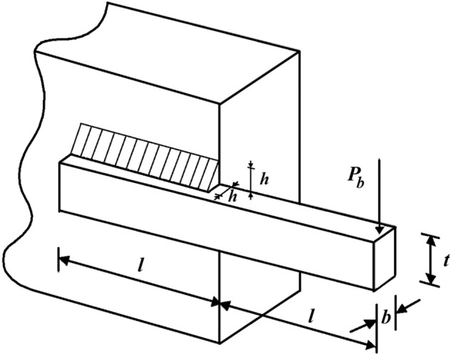
Schematic of welded beam design.
Table 10.
Performance of optimization algorithms in the design of welded beams.
| Algorithms | Optimum variables | Optimum cost | |||
|---|---|---|---|---|---|
| h | l | t | b | ||
| DTBO | 0.205730 | 3.470500 | 9.036600 | 0.205730 | 1.724900 |
| AVOA | 0.205936 | 3.473962 | 9.045661 | 0.205936 | 1.726578 |
| RSA | 0.144825 | 3.517514 | 8.934025 | 0.211832 | 1.674273 |
| MPA | 0.218678 | 3.513750 | 8.881413 | 0.225135 | 1.867986 |
| TSA | 0.205769 | 3.478321 | 9.044835 | 0.206017 | 1.729384 |
| WOA | 0.205884 | 3.478878 | 9.046000 | 0.206435 | 1.730721 |
| GWO | 0.197608 | 3.318376 | 10.00800 | 0.201596 | 1.824323 |
| MVO | 0.205817 | 3.475574 | 9.049972 | 0.205915 | 1.729194 |
| TLBO | 0.204900 | 3.539827 | 9.013294 | 0.210235 | 1.762968 |
| GSA | 0.147245 | 5.496235 | 10.01000 | 0.217943 | 2.177546 |
| PSO | 0.164335 | 4.036574 | 10.01000 | 0.223871 | 1.878014 |
| GA | 0.206693 | 3.639508 | 10.01000 | 0.203452 | 1.840211 |
Table 11.
Statistical results of optimization algorithms in the design of welded beams.
| Algorithms | Best | Mean | Worst | Std. Dev. | Median |
|---|---|---|---|---|---|
| DTBO | 1.724910 | 1.728057 | 1.730148 | 0.004332 | 1.727332 |
| AVOA | 1.726578 | 1.728851 | 1.729280 | 0.005128 | 1.727550 |
| RSA | 1.674273 | 1.705118 | 1.763902 | 0.017442 | 1.728144 |
| MPA | 1.867986 | 1.893952 | 2.018394 | 0.007968 | 1.885424 |
| TSA | 1.729384 | 1.730591 | 1.730826 | 0.000287 | 1.730549 |
| WOA | 1.730721 | 1.731893 | 1.732330 | 0.001161 | 1.731852 |
| GWO | 1.824323 | 2.236462 | 3.056641 | 0.325421 | 2.250856 |
| MVO | 1.729194 | 1.734452 | 1.746456 | 0.004881 | 1.732185 |
| TLBO | 1.762968 | 1.822671 | 1.878577 | 0.027619 | 1.825149 |
| GSA | 2.177546 | 2.551258 | 3.011943 | 0.256565 | 2.501997 |
| PSO | 1.878014 | 2.125086 | 2.326525 | 0.034916 | 2.102834 |
| GA | 1.840211 | 1.367289 | 2.040862 | 0.139871 | 1.941088 |
Figure 7.
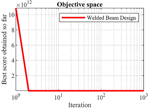
DTBO performance convergence curve for the welded beam design.
Conclusion and future works
This paper introduced a new stochastic human-based algorithm called Driving Training-Based Optimization (DTBO). The process of learning to drive in a driving school is the fundamental inspiration of the DTBO design. DTBO was mathematically modeled in three phases: (i) training by the driving instructor, (ii) patterning of students from instructor skills, and (iii) practice. Furthermore, we have shown the performance of DTBO in optimizing fifty-three objective functions of a group of unimodal, high-dimensional, fixed-dimensional multimodal, and IEE CEC2017. The results obtained from the implementation of DTBO in the objective functions to showed that DTBO has a high ability to exploit, explore, and balance them to perform powerfully in the optimization process.
The optimization results of the functions to showed the acceptable ability of DTBO to solve complex optimization problems.
To analyze the performance of DTBO, we compared its results with the performance of 11 well-known algorithms. A comparison of DTBO performance against competitor algorithms showed that the proposed DTBO, with better results, is more effective in optimizing and achieving optimal solutions and is much more competitive than the algorithms compared.
The use of DTBO in addressing two engineering design issues demonstrated the effective ability of the proposed approach in solving real-world applications. The authors offer several research pathways for future studies, including the development of binary and multi-objective versions of DTBO, which are among the particular study potentials of this paper. The application of DTBO in optimization problems in various sciences and real-world optimization challenges are other perspectives on the study of the proposed approach.
Although DTBO has provided acceptable results in solving the problems studied in this paper, there are some limitations to this method in other applications. The authors do not in any way claim that DTBO is the best optimizer in solving optimization problems because according to the concept of the NFL theorem, such a hypothesis is completely and definitively rejected. Therefore, DTBO may not be effective in solving some optimization applications. Furthermore, the main limitation of any metaheuristic algorithm, including DTBO, is that there is always the possibility that new optimization approaches may be developed in the future that perform better in the handling of optimization applications.
Author contributions
Conceptualization, M.D. and E.T.; methodology, P.T.; software, M.D.; validation, P.T. and M.D.; formal analysis, M.D.; investigation, P.T.; resources, E.T.; data curation, M.D.; visualization, P.T.; funding acquisition, E.T. All authors have read and agreed to the published version of the manuscript.
Funding
This research was funded by the Project of Specific Research of Faculty of Science, University of Hradec Králové, Czech Republic, Grant number 2104/2022-2023.
Data availability
All data generated or analyzed during this study are included directly in the text of this submitted manuscript. There are no additional external files with datasets.
Code availability
The source code of the DTBO algorithm is available at: https://uk.mathworks.com/matlabcentral/fileexchange/110755-driving-training-based-optimization.
Competing interests
The authors declare no competing interests.
Footnotes
Publisher's note
Springer Nature remains neutral with regard to jurisdictional claims in published maps and institutional affiliations.
References
- 1.Ray T, Liew KM. Society and civilization: An optimization algorithm based on the simulation of social behavior. IEEE Trans. Evol. Comput. 2003;7:386–396. doi: 10.1109/TEVC.2003.814902. [DOI] [Google Scholar]
- 2.Kaidi W, Khishe M, Mohammadi M. Dynamic levy flight chimp optimization. Knowl. Based Syst. 2022;235:107625. doi: 10.1016/j.knosys.2021.107625. [DOI] [Google Scholar]
- 3.Sergeyev YD, Kvasov D, Mukhametzhanov M. On the efficiency of nature-inspired metaheuristics in expensive global optimization with limited budget. Sci. Rep. 2018;8:1–9. doi: 10.1038/s41598-017-18940-4. [DOI] [PMC free article] [PubMed] [Google Scholar]
- 4.Iba K. Reactive power optimization by genetic algorithm. IEEE Trans. Power Syst. 1994;9:685–692. doi: 10.1109/59.317674. [DOI] [Google Scholar]
- 5.Wang J-S, Li S-X. An improved grey wolf optimizer based on differential evolution and elimination mechanism. Sci. Rep. 2019;9:1–21. doi: 10.1038/s41598-018-37186-2. [DOI] [PMC free article] [PubMed] [Google Scholar]
- 6.Wolpert DH, Macready WG. No free lunch theorems for optimization. IEEE Trans. Evol. Comput. 1997;1:67–82. doi: 10.1109/4235.585893. [DOI] [Google Scholar]
- 7.Kennedy, J. & Eberhart, R. Particle swarm optimization. In Proceedings of International Conference on Neural Networks’95, 1942–1948 (IEEE, 1995).
- 8.Yang X-S. Stochastic Algorithms: Foundations and Applications. SAGA 2009. Springer; 2009. Firefly algorithms for multimodal optimization; pp. 169–178. [Google Scholar]
- 9.Karaboga, D. & Basturk, B. Artificial bee colony (ABC) optimization algorithm for solving constrained optimization problems. In Foundations of Fuzzy Logic and Soft Computing. IFSA 2007. Lecture Notes in Computer Science, 789–798 (Springer, Berlin, 2007).
- 10.Dorigo M, Stützle T. Handbook of Metaheuristics, Chap. Ant Colony Optimization: Overview and Recent Advances. Springer; 2019. pp. 311–351. [Google Scholar]
- 11.Kaur S, Awasthi LK, Sangal AL, Dhiman G. Tunicate swarm algorithm: A new bio-inspired based metaheuristic paradigm for global optimization. Eng. Appl. Artif. Intell. 2020;90:103541. doi: 10.1016/j.engappai.2020.103541. [DOI] [Google Scholar]
- 12.Abualigah L, Elaziz MA, Sumari P, Geem ZW, Gandomi AH. Reptile search algorithm (RSA): A nature-inspired meta-heuristic optimizer. Expert Syst. Appl. 2022;191:116158. doi: 10.1016/j.eswa.2021.116158. [DOI] [Google Scholar]
- 13.Mirjalili S, Lewis A. The whale optimization algorithm. Adv. Eng. Softw. 2016;95:51–67. doi: 10.1016/j.advengsoft.2016.01.008. [DOI] [Google Scholar]
- 14.Jiang Y, Wu Q, Zhu S, Zhang L. Orca predation algorithm: A novel bio-inspired algorithm for global optimization problems. Expert Syst. Appl. 2022;188:116026. doi: 10.1016/j.eswa.2021.116026. [DOI] [Google Scholar]
- 15.Faramarzi A, Heidarinejad M, Mirjalili S, Gandomi AH. Marine predators algorithm: A nature-inspired metaheuristic. Expert Syst. Appl. 2020;152:113377. doi: 10.1016/j.eswa.2020.113377. [DOI] [Google Scholar]
- 16.Trojovský P, Dehghani M. Pelican optimization algorithm: A novel nature-inspired algorithm for engineering applications. Sensors. 2022;22:855. doi: 10.3390/s22030855. [DOI] [PMC free article] [PubMed] [Google Scholar]
- 17.Coufal P, Hubálovský Š, Hubálovská M, Balogh Z. Snow leopard optimization algorithm: A new nature-based optimization algorithm for solving optimization problems. Mathematics. 2021;9:2832. doi: 10.3390/math9212832. [DOI] [Google Scholar]
- 18.Mirjalili S, Mirjalili SM, Lewis A. Grey wolf optimizer. Adv. Eng. Softw. 2016;69:46–61. doi: 10.1016/j.advengsoft.2013.12.007. [DOI] [Google Scholar]
- 19.Abdollahzadeh B, Gharehchopogh FS, Mirjalili S. Artificial gorilla troops optimizer: A new nature-inspired metaheuristic algorithm for global optimization problems. Int. J. Intell. Syst. 2021;36:5887–5958. doi: 10.1002/int.22535. [DOI] [Google Scholar]
- 20.Abdollahzadeh B, Gharehchopogh FS, Mirjalili S. African vultures optimization algorithm: A new nature-inspired metaheuristic algorithm for global optimization problems. Comput. Ind. Eng. 2021;158:107408. doi: 10.1016/j.cie.2021.107408. [DOI] [Google Scholar]
- 21.Shayanfar H, Gharehchopogh FS. Farmland fertility: A new metaheuristic algorithm for solving continuous optimization problems. Appl. Soft Comput. 2018;71:728–746. doi: 10.1016/j.asoc.2018.07.033. [DOI] [Google Scholar]
- 22.Ghafori S, Gharehchopogh FS. Advances in spotted hyena optimizer: A comprehensive survey. Arch. Comput. Methods Eng. 2022;Early Access:1–22. [Google Scholar]
- 23.Gharehchopogh FS. Advances in tree seed algorithm: A comprehensive survey. Arch. Comput. Methods Eng. 2022;Early Access:1–24. doi: 10.1007/s11831-022-09804-w. [DOI] [PMC free article] [PubMed] [Google Scholar]
- 24.Goldberg DE, Holland JH. Genetic algorithms and machine learning. Mach. Learn. 1988;3:95–99. doi: 10.1023/A:1022602019183. [DOI] [Google Scholar]
- 25.Storn R, Price K. Differential evolution-a simple and efficient heuristic for global optimization over continuous spaces. J. Global Optim. 1997;11:341–359. doi: 10.1023/A:1008202821328. [DOI] [Google Scholar]
- 26.Kirkpatrick S, Gelatt CD, Vecchi MP. Optimization by simulated annealing. Science. 1983;220:671–680. doi: 10.1126/science.220.4598.671. [DOI] [PubMed] [Google Scholar]
- 27.Rashedi E, Nezamabadi-Pour H, Saryazdi S. Gsa: A gravitational search algorithm. Inf. Sci. 2009;179:2232–2248. doi: 10.1016/j.ins.2009.03.004. [DOI] [Google Scholar]
- 28.Eskandar H, Sadollah A, Bahreininejad A, Hamdi M. Water cycle algorithm-a novel metaheuristic optimization method for solving constrained engineering optimization problems. Comput. Struct. 2012;110:151–166. doi: 10.1016/j.compstruc.2012.07.010. [DOI] [Google Scholar]
- 29.Mirjalili S, Mirjalili SM, Hatamlou A. Multi-verse optimizer: A nature-inspired algorithm for global optimization. Neural Comput. Appl. 2016;27:495–513. doi: 10.1007/s00521-015-1870-7. [DOI] [Google Scholar]
- 30.Tahani M, Babayan N. Flow regime algorithm (FRA): A physics-based meta-heuristics algorithm. Knowl. Inf. Syst. 2019;60:1001–1038. doi: 10.1007/s10115-018-1253-3. [DOI] [Google Scholar]
- 31.Wei Z, Huang C, Wang X, Han T, Li Y. Nuclear reaction optimization: A novel and powerful physics-based algorithm for global optimization. IEEE Access. 2019;7:66084–66109. doi: 10.1109/ACCESS.2019.2918406. [DOI] [Google Scholar]
- 32.Dehghani M, et al. A spring search algorithm applied to engineering optimization problems. Appl. Sci. 2020;10:6173. doi: 10.3390/app10186173. [DOI] [Google Scholar]
- 33.Faramarzi A, Heidarinejad M, Stephens B, Mirjalili S. Equilibrium optimizer: A novel optimization algorithm. Knowl. Based Syst. 2020;191:105190. doi: 10.1016/j.knosys.2019.105190. [DOI] [Google Scholar]
- 34.Moghdani R, Salimifard K. Volleyball premier league algorithm. Appl. Soft Comput. 2018;64:161–185. doi: 10.1016/j.asoc.2017.11.043. [DOI] [Google Scholar]
- 35.Dehghani M, Mardaneh M, Guerrero JM, Malik O, Kumar V. Football game based optimization: An application to solve energy commitment problem. Int. J. Intell. Eng. Syst. 2020;13:514–523. [Google Scholar]
- 36.Zeidabadi FA, Dehghani M. Poa: Puzzle optimization algorithm. Int. J. Intell. Eng. Syst. 2022;15:273–281. [Google Scholar]
- 37.Kaveh A, Zolghadr A. A novel meta-heuristic algorithm: Tug of war optimization. Iran Univ. Sci. Technol. 2016;6:469–492. [Google Scholar]
- 38.Rao RV, Savsani VJ, Vakharia D. Teaching-learning-based optimization: A novel method for constrained mechanical design optimization problems. Comput. Aided Des. 2011;43:469–492. doi: 10.1016/j.cad.2010.12.015. [DOI] [Google Scholar]
- 39.Moosavi SHS, Bardsiri VK. Poor and rich optimization algorithm: A new human-based and multi populations algorithm. Eng. Appl. Artif. Intell. 2019;86:165–181. doi: 10.1016/j.engappai.2019.08.025. [DOI] [Google Scholar]
- 40.Mousavirad SJ, Ebrahimpour-Komleh H. Human mental search: A new population-based metaheuristic optimization algorithm. Appl. Intell. 2017;47:850–887. doi: 10.1007/s10489-017-0903-6. [DOI] [Google Scholar]
- 41.Dehghani M, et al. A new doctor and patient optimization algorithm: An application to energy commitment problem. Appl. Sci. 2020;10:5791. doi: 10.3390/app10175791. [DOI] [Google Scholar]
- 42.Abdollahzadeh B, Gharehchopogh FS. A multi-objective optimization algorithm for feature selection problems. Eng. Comput. 2021;Early Access:1–19. [Google Scholar]
- 43.Benyamin A, Farhad SG, Saeid B. Discrete farmland fertility optimization algorithm with metropolis acceptance criterion for traveling salesman problems. Int. J. Intell. Syst. 2021;36:1270–1303. doi: 10.1002/int.22342. [DOI] [Google Scholar]
- 44.Mohmmadzadeh H, Gharehchopogh FS. An efficient binary chaotic symbiotic organisms search algorithm approaches for feature selection problems. J. Supercomput. 2021;77:9102–9144. doi: 10.1007/s11227-021-03626-6. [DOI] [Google Scholar]
- 45.Mohmmadzadeh H, Gharehchopogh FS. Feature selection with binary symbiotic organisms search algorithm for email spam detection. Int. J. Inf. Technol. Decis. Mak. 2021;20:469–515. doi: 10.1142/S0219622020500546. [DOI] [Google Scholar]
- 46.Zaman HRR, Gharehchopogh FS. An improved particle swarm optimization with backtracking search optimization algorithm for solving continuous optimization problems. Eng. Comput. 2021;Early Access:1–35. [Google Scholar]
- 47.Gharehchopogh FS, Farnad B, Alizadeh A. A modified farmland fertility algorithm for solving constrained engineering problems. Concurr. Comput. Pract. Exp. 2021;Early Access:e6310. [Google Scholar]
- 48.Gharehchopogh FS, Abdollahzadeh B. An efficient harris hawk optimization algorithm for solving the travelling salesman problem. Cluster Comput. 2021;Early Access:1–25. [Google Scholar]
- 49.Mohmmadzadeh H, Gharehchopogh FS. A multi-agent system based for solving high-dimensional optimization problems: A case study on email spam detection. Int. J. Commun. Syst. 2021;34:e4670. [Google Scholar]
- 50.Gharehchopogh FS. An improved tunicate swarm algorithm with best-random mutation strategy for global optimization problems. J. Bionic Eng. 2022;Early Access:1–26. [Google Scholar]
- 51.Goldanloo MJ, Gharehchopogh FS. A hybrid obl-based firefly algorithm with symbiotic organisms search algorithm for solving continuous optimization problems. J. Supercomput. 2022;78:3998–4031. doi: 10.1007/s11227-021-04015-9. [DOI] [Google Scholar]
- 52.Mohmmadzadeh H, Gharehchopogh FS. A novel hybrid whale optimization algorithm with flower pollination algorithm for feature selection: Case study email spam detection. Comput. Intell. 2021;37:176–209. doi: 10.1111/coin.12397. [DOI] [Google Scholar]
- 53.Yao X, Liu Y, Lin G. Evolutionary programming made faster. IEEE Trans. Evol. Comput. 1999;3:82–102. doi: 10.1109/4235.771163. [DOI] [Google Scholar]
- 54.Awad, N., Ali, M., Liang, J., Qu, B. & Suganthan, P. Evaluation criteria for the cec 2017 special session and competition on single objective real-parameter numerical optimization. Tech. Rep., Kyungpook National University: Daegu, South Korea (2016).
- 55.Wilcoxon F. Break throughs in Statistics, chap. Individual Comparisons by Ranking Methods. Springer; 1992. pp. 196–202. [Google Scholar]
- 56.Kannan B, Kramer SN. An augmented lagrange multiplier based method for mixed integer discrete continuous optimization and its applications to mechanical design. J. Mech. Des. 1994;116:405–411. doi: 10.1115/1.2919393. [DOI] [Google Scholar]
Associated Data
This section collects any data citations, data availability statements, or supplementary materials included in this article.
Data Availability Statement
All data generated or analyzed during this study are included directly in the text of this submitted manuscript. There are no additional external files with datasets.
The source code of the DTBO algorithm is available at: https://uk.mathworks.com/matlabcentral/fileexchange/110755-driving-training-based-optimization.