Figure 3.

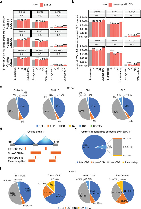
Distributions of structural variations among 3D genome architectures. a) Density of SVs (insertions, deletions, and duplications) in A/B compartments and CDBs. The density of SVs is the number of SVs divided by the length of each chromosome region. Gray bars represent background sequence and show the density of SVs on the chromosomes. Red bars show the density of SVs on the different chromosome regions, including A/B compartments, CDs, and CDBs. Enrichment tests were performed via R's prop. test, which was evaluated by comparing the proportion of SVs falling in the region of interest and the proportion of the length of the region of interest in the whole genome. ****p ≤ 0.0001, ***p ≤ 0.001, **p ≤ 0.01, *p ≤ 0.05. b) The density of cancer‐specific SVs (insertions, deletions, and duplications) in A/B compartments and TAD boundary. Cancer‐specific SVs refer to those occurring in BxPC3 (or PANC1) but not in HPDE6C7. Enrichment tests were performed via R's prop. test, which was evaluated by comparing the proportion of SVs falling in the region of interest and the proportion of the length of the region of interest in the whole genome. ****p ≤ 0.0001, ***p ≤ 0.001, **p ≤ 0.01, *p ≤ 0.05. c) The proportion of different types of cancer‐specific SVs (less than 2 Mb length) in different A/B compartment regions of BxPC3. d) Schematic diagram of SV categories according to the position relationship between the breakpoint of cancer‐specific SVs and the CD boundary. e) Number and percentage of four different specific SV types in BxPC3 according to (d). f) Number and percentage of different types of four categories of cancer‐specific SVs in BxPC3 according to (d).