Temperature Controls eDNA Persistence across Physicochemical Conditions in Seawater

Abstract

Environmental DNA (eDNA) quantification and sequencing are emerging techniques for assessing biodiversity in marine ecosystems. Environmental DNA can be transported by ocean currents and may remain at detectable concentrations far from its source depending on how long it persist. Thus, predicting the persistence time of eDNA is crucial to defining the spatial context of the information derived from it. To investigate the physicochemical controls of eDNA persistence, we performed degradation experiments at temperature, pH, and oxygen conditions relevant to the open ocean and the deep sea. The eDNA degradation process was best explained by a model with two phases with different decay rate constants. During the initial phase, eDNA degraded rapidly, and the rate was independent of physicochemical factors. During the second phase, eDNA degraded slowly, and the rate was strongly controlled by temperature, weakly controlled by pH, and not controlled by dissolved oxygen concentration. We demonstrate that marine eDNA can persist at quantifiable concentrations for over 2 weeks at low temperatures (≤10 °C) but for a week or less at ≥20 °C. The relationship between temperature and eDNA persistence is independent of the source species. We propose a general temperature-dependent model to predict the maximum persistence time of eDNA detectable through single-species eDNA quantification methods.

Short abstract

Organisms shed trace amounts of DNA into the environment (eDNA). Quantification and sequencing of eDNA can inform the distribution and diversity of biological communities. Estimating the temporal persistence of eDNA is fundamental to constraining its source. This study (1) finds that temperature strongly controls the maximum persistence time of eDNA in the ocean and (2) proposes a model to estimate the maximum persistence time of eDNA as it relates to seawater temperature.

Introduction

Anthropogenic impacts are causing species extinctions and population declines globally.¹⁻³ Molecular biology methods accelerate the pace at which vulnerable biological communities are characterized to inform conservation and ecosystem restoration efforts.^4,5 Environmental DNA (eDNA) sequencing and quantification complement conventional methods for assessing biodiversity and the distribution of invasive and ecologically important species in marine habitats.⁶⁻¹⁰ However, the utility of eDNA methods hinges on understanding the factors that control the distribution and abundance of eDNA across spatiotemporal scales.¹¹

Aqueous eDNA is DNA that is dissolved in solution or associated with larger suspended particles, such as cells, organelles, or aggregates.¹² Animal eDNA may be shed into the environment through several processes, and the shedding rate depends on factors like biomass, metabolic rate, ontogeny, and activity.¹³⁻¹⁹ Once shed from an animal, eDNA changes from intracellular to subcellular states.²⁰⁻²² eDNA degrades at rates influenced by physicochemical and biotic factors, and the relative influence of these factors may depend on its state.^12,22−25 Before completely degrading into short fragments that molecular methods cannot detect, marine eDNA can be transported away from its source by ocean currents.^25,26 Determining how the persistence of eDNA is controlled by physicochemical conditions is vital to constraining when and where it was shed from a source organism. This knowledge is essential to define the spatiotemporal resolution of the ecological information derived from eDNA quantification and sequencing.

Experimental studies using freshwater and marine animals have established that eDNA degrades beyond the detection limit of PCR-based methods over timescales spanning hours to weeks. These studies have indicated that temperature, pH, and dissolved oxygen concentration may influence the degradation rate and, thus, the persistence of environmental DNA. Temperature controls the degradation rate of eDNA shed from diverse organisms.^{17,21,24,27−33} Higher temperatures increase the kinetics of many processes responsible for DNA degradation, including cell and organelle lysis, hydrolysis and oxidation of DNA molecules, and breakdown by extracellular enzymes. The stability of the DNA molecules is affected by pH.³⁴⁻³⁶ Consistently, experiments have indicated that the rate of eDNA degradation is also affected by pH.^27,29,37,38 However, these experimental inquiries have been limited to freshwater systems where pH ranges widely, from 5.0 to 9.0. No study has experimentally tested the effect of pH on eDNA degradation in seawater, which has a narrower range between 7.5 and 8.3.

Dissolved oxygen concentration (hereafter abbreviated as [DO]) is another potentially important physicochemical parameter that has received comparatively little attention. Dissolved oxygen concentration is biologically relevant due to its importance to microbial metabolism. Oxygen is also chemically relevant due to the susceptibility of DNA molecules to oxidation. Only one study has experimentally manipulated [DO] to determine its effect on eDNA decay in seawater.²³ That study found that the degradation rate of eDNA was slower at a dissolved oxygen saturation of 20% versus 55%. To fully determine the effect of [DO] on eDNA degradation, it is necessary to perform experiments across the range of oxygenation states in marine ecosystems, from fully oxygenated to nearly anoxic.

Temperature, pH, and [DO] vary considerably with location and depth in the open ocean. Temperature decreases from ∼30 °C in the tropical surface ocean to near freezing in the deep sea, and pH typically changes with depth from approximately 8.3 to 7.5.³⁹ Seawater is usually nearly saturated with oxygen in the surface ocean. Oxygen saturation decreases to a minimum at mesopelagic depths and increases with higher solubility at lower temperatures in the deep sea.⁴⁰ Considering the potentially interactive effects of these abiotic factors on the persistence of marine eDNA is necessary when applying eDNA methodologies to study ocean biodiversity.

Here, we test the relative effects of temperature, pH, and [DO] on the degradation rate of eDNA across conditions that reflect the subtropical open ocean, spanning near-surface waters to the deep sea. We developed an experimental setup that allows tight control of physicochemical conditions and produces reproducible results. We used the deep-sea coral Desmophyllum pertusum (Linnaeus 1758) as the source of eDNA. D. pertusum is hereafter referred to as Lophelia for consistency with abundant literature that uses its synonymized name Lophelia pertusa.(41)Lophelia is an ecologically important reef-forming coral with a cosmopolitan distribution in cold and deep waters of the Atlantic and Pacific Oceans.^42,43 We hypothesized that temperature, pH, and [DO] would have interactive effects controlling the degradation rate of eDNA.

Materials and Methods

Experimental Conditions

To test our hypothesis, we conducted eDNA degradation experiments under 11 fixed combinations of temperature (set to either 4, 10, or 20 °C), [DO] (set to either nearly anoxic, 0.1 mg/L; half saturated, 3.6 mg/L; or fully saturated, 7.2 mg/L), and pH (set to either 7.6, 7.9, or 8.2). These discrete sets of physicochemical conditions were chosen to reflect the range of conditions found in the subtropical open ocean, spanning from near-surface waters to the deep sea. Each set of conditions was investigated in duplicate experiments (22 experiments in total) to assess the reproducibility in estimating the eDNA degradation rate. We maintained these conditions at target values throughout the experiments with accuracy (Figure 1).

Figure 1.

(A) Matrix of target conditions for 11 combinations of temperature, pH, and [DO] investigated to determine the persistence of eDNA from the coral Lophelia among a range of marine physicochemical states. Two replicate experiments were conducted for each combination of temperature, pH, and [DO]. At 20 °C temperature, half- and fully saturated oxygen experiments (shaded light blue) represent conditions characteristic of subtropical near-surface environments. At 4 °C temperature, half-saturated experiments (shaded dark blue) represent conditions characteristic of the deep-sea environment. The remaining cells (shaded blue) represent other conditions characteristic of the global open and deep ocean. (B) Schematic example of experimental conditions. Compressed air and nitrogen gas flow rates were adjusted to reach the target [DO]. Small doses of 0.5 M HCl were automatically administered to the tanks when target pH values were exceeded. Physicochemical measurements were monitored by suspending probes in the tanks. Caps were secured with O-rings to control the oxygen concentration in the above headspace. All tubing and probes were placed through small openings in these caps. A photograph of the experimental setup is presented in Figure S1. (C) Measurements of temperature, pH, and [DO] over the 22 eDNA degradation experiments. Points indicate individual measurements, and paths are drawn through daily averages. All measurements were recorded daily and at each sampling time point. Temperature measurements were made using a laser thermometer. pH and [DO] measurements were made with probes.

Experimental Setup

Experiments were conducted in a controlled-temperature room (KE2 Therm Solutions Inc., Washington, MO, USA) set to the target temperature. The ambient temperature room was monitored using a HOBO data logger (Onset Computer Corporation, Bourne, MA, USA). The temperature of each tank was also measured daily and at each sampling time point using an Etekcity infrared laser thermometer (Vesync Co., Anaheim, CA, USA).

Experiments were conducted in opaque polypropylene carboys in the controlled-temperature room with no windows, and artificial fluorescent lights were on only during sampling. These conditions removed the potential effect of UV light on the eDNA degradation rate in the experiments. Natural levels of UV radiation from sunlight have not been found to affect marine eDNA degradation significantly.⁴⁴ Therefore, eliminating UV light should have a negligible effect on interpreting results from experiments that may reflect conditions in the surface ocean (high-pH and oxygenated), where UV radiation penetrates.⁴⁵

We continuously monitored the pH using a BlueLab pH Controller Connect System (BlueLab, New Zealand) with a single-junction pH electrode (Oakton, Vernon Hills, IL, USA) and an RTD temperature probe (BlueLab) for automatic temperature compensation. Target pH values were maintained by automated dosing with small volumes of 0.5 M hydrochloric acid whenever the controller pH reading exceeded 0.1 pH unit over the target value (approximately hourly). We manually added small volumes (<5 mL) of 0.5 M sodium hydroxide if the pH reading dropped below 0.1 pH unit of the target value. Duplicate, small-volume samples (∼50 mL) were removed at each sampling time point to obtain independent pH measurements using an Orion PerpHect Log R meter (Thermo Fisher Scientific, Waltham, MA, USA) with a single-junction pH electrode (Oakton). The pH monitoring systems were calibrated at the start of each experiment using a three-point calibration with pH 4.01, 7.00, and 10.01 solutions (Oakton). The pH meter used for daily sampling measurements was calibrated before each measurement using two-point calibration with pH 7.00 and 10.01 solutions (Oakton). pH measurements were temperature-compensated manually by setting the monitor to the ambient temperature of the room.

We controlled the [DO] by manipulating the flow rates of compressed air and high-purity nitrogen gas. Compressed air and nitrogen flow rates were set with Aalborg GFC Mass Flow Controllers (Aalborg, Orangeburg, NY, USA). Before each experiment, gas flow rates were independently verified using a soap film bubble flow meter. Gasses were delivered to each experimental tank using independent gas lines capped with air stones placed at the bottom (Figure 1). Dissolved oxygen concentrations and oxidative reductive potential (ORP) were monitored within the experimental tanks and recorded daily and at each sampling time point with Pinpoint II Dissolved Oxygen and Pinpoint ORP monitors, respectively (American Marine, Ridgefield, CT, USA). Dissolved oxygen concentration and ORP monitors were calibrated at the start of each experiment, following the manufacturer’s instructions. The [DO] monitors were calibrated to atmospheric oxygen concentration. The ORP monitors were calibrated using the manufacturer-supplied 400 ORP AgCl reference standard (American Marine).

eDNA Degradation Experiments

For each experiment, 42 L of artificial seawater at 35 PSU salinity were prepared in a polypropylene carboy (Foxx Life Sciences, Salem, NH, USA) using the B-Ionic Artificial Seawater (ASW) System (ESV Aquarium Products, Hicksville, NY, USA). Seawater was prepared with ultrapure deionized water using a Milli-Q system with an attached LC-Pak Polisher (Millipore Sigma, Burlington, MA, USA). The LC-Pak Polisher removes trace organics from water. We chose to make ASW from Milli-Q water to restrict organic material sources to the B-Ionic ASW components and our eDNA source.

We prepared a tissue homogenate from freshly frozen Lophelia fragments as the source of eDNA. Fragments approximately 10 cm in length with 8–10 polyps were collected at two sites at ∼700 and ∼760 m depth at the Richardson Reef Complex off the coast of South Carolina, USA (31.98°N, 77.41°W and 31.88°N, 77.37°W, respectively). Collection details are presented in the Supplementary Methods. Lophelia tissue was removed from the skeleton with a strong stream of ASW using a water jet dental flosser. The resulting mixture of tissue and ASW was collected in a sterile Whirl-Pak. This mixture was homogenized using a FisherBrand 150 rotor–stator homogenizer with a 5 mm fine-sawtooth probe (Thermo Fisher Scientific, Waltham, MA, USA). The homogenate was aliquoted into 15 mL sterile centrifuge tubes (Celltreat, Pepperell, MA, USA), frozen, and stored at −80 °C. One aliquot was thawed on ice immediately before each experiment. Details about the preparation and choice of source eDNA are presented in the Supplementary Methods.

Between 12 and 15 mL of tissue homogenate was added to each tank at the beginning of each experiment. The concentration was adjusted based on the measured concentration of coral eDNA in each preparation to keep starting concentrations consistent among experiments (see Supplementary Methods). From this point onwards, seawater from each experiment was serially sampled at increasing time intervals to quantify the concentration of coral eDNA over time. The first sample was taken between 30 and 45 min after adding the homogenate to allow mixing. After conducting pilot experiments, we determined that sampling over 8 days was sufficient for experiments at 20 °C since the limit of quantification of our qPCR assay was reached in less than a week. However, this timeframe was insufficient to capture the entire degradation process at lower temperatures. Thus, sampling for experiments at 10 and 4 °C was conducted less frequently over the first 2 days and extended to 17 days. Sampling time points for each experiment are shown in Figure 2. We sampled coral eDNA by filtering approximately 1 L of water (mean = 1008 mL; SD = 74 mL; range = 404 to 1145 mL) through a 0.22 μm pore-size polyethersulfone Sterivex filter (Millipore-Sigma). Water was pumped through the filter using an L/S peristaltic pump, Easy-Load II pump heads, and L/S 15 high-performance precision tubing (Masterflex, Vernon Hills, IL, USA). The pump was set to a rate of 100 RPM. The tubing was primed with tank water before a filter was attached. The effluent from each filtered sample was weighed using a balance to adjust measured concentrations of eDNA by mass (in g) of water filtered. Any water remaining in the tubing was pumped back into the experimental tanks once filtration was complete and the filter was removed. Following filtration, Sterivex filters were stored in sterile Whirl-Pak bags and frozen at −80 °C immediately after eDNA filtration until DNA extraction, which occurred within 1 month.

Figure 2.

Degradation of Lophelia eDNA in 22 experiments among a range of marine physicochemical states. eDNA concentration was measured as the concentration of a 154 base pair fragment of the Lophelia mitochondrial COI gene. The concentration of eDNA (y-axis) is plotted against time (x-axis). The y-axis is natural-log scaled. Different colors represent the two experimental replicates at each experimental condition. Points represent the average of three qPCR replicate measurements for two samples at a given time point. Lines represent the fit to a biphasic model. Thin lines connecting points to the line of best fit represent the distance from the observed to the fitted values at each time point (the residuals). Panels are arranged by temperature (descending top to bottom) and [DO] (increasing left to right). Values shown on top of each panel indicate the target experimental conditions. Points below the limit of quantification of the qPCR assay (77.8 copies/reaction or 13 copies/mL seawater filtered) are not plotted. The dashed line indicates the limit of quantification.

DNA Extraction and Quantitative PCR

DNA was extracted from each filter using a Qiagen DNEasy Blood & Tissue Kit (Hilden, Germany) following methods initially developed by Spens et al. with modifications described in Govindarajan et al.^46,47 The DNA was eluted in two separate volumes of 50 μL of AE buffer for a total volume of 100 μL per extraction. The total concentration of DNA in each extract was quantified using the Qubit 1X High-Sensitivity Double-Stranded DNA Assay (Thermo Fisher Scientific, Waltham, MA, USA). The average DNA concentration was 3.40 ng/μL, and the range was from <0.1 (too low to quantify) to 52.0 ng/μL. After this assay, the DNA was stored frozen at −20 °C.

We developed a new qPCR assay to amplify and quantify a 154 base pair fragment of the Lophelia mitochondrial COI gene (Lop-COI) using primers that match the COI gene of caryophylliid corals. The forward primer sequence is 5′-CTGGGGGACGATCATCTTTA-3′, and the reverse primer sequence is 5′-TGTTTAATCGGGGGAAAGC-3′. Primers were synthesized by Eurofins Genomics (Louisville, KY, USA), purified by standard desalting, and normalized at 100 μM in TE buffer (pH 8.0). Quantitative PCR reactions were performed in 20 μL volumes using the Quantabio PerfecTa SYBR Green Fastmix (Beverly, MA, USA) and a Qiagen RotorGene 6000 Thermal Cycler with either the 72-well or 36-well ring. We used clear Qiagen 0.1 mL four-strip tubes (for a 72-well ring) or 0.2 mL single tubes (for a 36-well ring) designed for the RotorGene. DNA extracts were diluted 10-fold in Buffer AE (Qiagen, Germany), and 6 μL of this dilution was used in each reaction (effectively 0.6 μL of DNA template). Primer stocks in TE buffer were diluted to 10 μM using molecular-grade water, and 6 pmol of both the forward and reverse primers were added to each reaction for a final concentration of 300 nM for each primer. We used molecular-grade water to complete the 20 μL volume of each reaction. Cycling conditions were as follows: initial denaturation at 95 °C for 10 min, then 35 cycles of denaturation at 95 °C for 15 s, annealing at 55 °C for 15 s, and elongation at 72 °C for 20 s. Amplification was followed by melting curve analysis and conducted with pre-melt conditioning at 72 °C for 90 s followed by a ramp from 72 to 95 °C with holds of 5 s per 0.5 °C increase in temperature. The details regarding primer design and qPCR assay optimization are presented in the Supplementary Methods. The qPCR assay’s quantification (LOQ) and detection limits (LOD) were calculated and visualized using code adapted from Klymus et al.⁴⁸ (see the Supplementary Methods for further details). The LOQ was determined to be 77.8 copies per reaction, equivalent to 13 copies/mL of seawater filtered using our sampling and eDNA extraction methods. The LOD with three qPCR replicates is 3.4 copies per reaction or 0.6 copies/mL of seawater filtered.

Each qPCR run consisted of 19 samples in triplicate, 4 10-fold dilutions of purified plasmids containing the target fragment (778,000 to 778 copies per reaction or 130,000 to 130 copies/mL seawater filtered) in triplicate, and 3 PCR negative controls. On average, each replicate qPCR reaction analyzed 6 mL (SD = 1.3 mL) of seawater. A sample was determined to have amplified if the characteristic exponential amplification curve was visualized in the log(RFU) and C_q value graph and if there was a distinct peak in the melting curve at 78 °C, which corresponded to the peak of the plasmid standard PCR products. The C_q threshold was set using the auto-threshold setting in RotorGene software. The amplified samples’ concentrations were determined by fitting the line of best fit to the standard curve in each run. The standard curves’ average R² and doubling efficiencies for the 33 qPCR runs were 0.99236 ± 0.01502 (SD) and 85.4 ± 4.7% (SD), respectively. The high R² of these calibration curves demonstrates that the linear dynamic range spanned the full range of DNA concentrations examined, from the highest DNA concentrations of our standards to the LOQ. The DNA concentrations from all experimental samples above the LOQ were bracketed by this range. The average slope of the standard curves was −3.7391 ± 0.155 (SD) C_q per order of magnitude decrease in concentration, and the average intercept was 7.4540 ± 2.5069 (SD) C_q.

Contamination Controls

Before each experiment, tanks were sterilized with a solution of 10% household bleach (6% sodium hypochlorite) and deionized water and were subsequently rinsed with Milli-Q water. Sampling tubes (Cole Parmer, Antylia Scientific, Vernon Hills, IL, USA) were sterilized by pumping a 10% bleach solution through them for 15 min and subsequently rinsed with at least 1 L of Milli-Q water. Luer fittings, air stones, and air stone tubings were sterilized by soaking in 10% bleach for at least an hour and rinsed by soaking in Milli-Q water. Temperature, pH, [DO], and ORP probes were rinsed thoroughly with Milli-Q water. All tubing and probe wiring exteriors were wiped with 10% bleach followed by Milli-Q water before placing them in the tanks. Experimental controls (42 L of ASW) without added tissue homogenate were conducted simultaneously with each set of degradation experiments (up to four at once). The physicochemical conditions in these controls were set and maintained in the same way as the degradation experiments. This tank was sampled at each time point alongside the experiments, serving as a sampling negative control to monitor for contamination during sampling. Sampling negative control samples were processed similarly to the experimental samples in all subsequent laboratory steps. All laboratory work was conducted in a laboratory adjacent to but separated from the controlled-temperature room where the experiments were conducted. DNA extractions were conducted at a dedicated bench where no tissue DNA extractions had occurred. Pipettes for eDNA extraction were wiped with 10% bleach solution and UV-irradiated before each set of extractions. In each set of extractions, an extraction negative control was also processed to monitor for contamination at this step. Quantitative PCR (qPCR) preparation was conducted in a My-PCR Prep Station (Mystaire, Creedmoor, NC, USA) hood with positive airflow, air filtration through a HEPA filter, and an overhead UV lamp. Sterile filter tips were used at all stages of laboratory work. qPCR was conducted at a bench for qPCR cycling and post-PCR work. qPCR products were disposed of in this lab area, and PCR products were not brought into any other part of the lab.

Of all sampling negative controls, extraction negative controls, and PCR negative controls measured, a single qPCR replicate from one extraction negative control and one PCR negative control amplified (both below the LOQ). The estimated concentrations of these two samples were 9.6 and 5.6 copies per reaction, or 1.6 and 0.9 copies/mL seawater filtered, respectively. No replicates from any other triplicates of the 204 negative control samples amplified. This results in a false positive rate of just 0.9% if the amplification of a single qPCR triplicate at concentrations below the LOQ is considered a positive signal. Thus, we have high confidence that our experiments were free of contamination that would affect the interpretation of our results.

Statistical Analyses

All data analyses and visualizations were conducted using R version 4.1.0 (R Core Team) in RStudio. Plots were created with ggplot2⁴⁹ and edited in Adobe Illustrator. Decay models were fitted to the mean of qPCR triplicates for each eDNA sample to determine decay rate constants for each experiment. All three replicates were averaged in all cases, and we did not remove any potential outlying qPCR replicates. We only analyzed experimental time points where the mean concentration of the three qPCR triplicates was above the LOQ.

A simple exponential model was fit as a linear model to natural log-transformed data from each experiment using the lm function. The linear model is defined as LN(Y) = – kt + LN(Y₀). Here, the slope is mathematically equivalent to an exponential model’s decay rate constant, k. A decreasing rate of eDNA degradation over time has been observed in other studies.^28,32,50,51 Therefore, we also fit a biphasic model to natural log-transformed data as two linear models, allowing for a change in the decay rate constant over time. The biphasic linear model is defined as 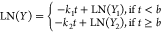, where k₁ is the initial decay rate constant and k₂ is the second decay rate constant defined for time points, t, after a breakpoint, b, in the model. The natural log of Y₁ and Y₂ are the intercepts of each model (in natural log eDNA copies per reaction) during the initial and second phases of eDNA decay, respectively. The optimal breakpoint time for each model was estimated using the R package segmented.⁵² The number of breakpoints to be estimated was set to 1, and the starting value for estimation was set to 24 h.

To avoid overparameterization, we chose to fit a biphasic model over other more complex nonlinear models. This model choice also allows for direct comparisons of the decay rate constant estimates from each phase among experiments and the decay rate constants reported in other studies. For each experiment, we calculated the log-likelihood and Bayesian information criterion (BIC) of the linear and biphasic models. A likelihood ratio test and comparison of BICs were conducted to determine which model was better at describing the data.

We fit a linear mixed model (LMM) on eDNA concentrations from each phase separately and considered the influence of temperature, pH, [DO], and relevant covariates on eDNA degradation. One outlier experiment, which exhibited a breakpoint in the biphasic model that was substantially later than the others (discussed more in depth in the Results and Discussion section), was omitted from these analyses. Linear mixed models were fit to the data using the R package lme4.⁵³ The significance of each coefficient was assessed with t tests using Satterthwaite’s method to determine degrees of freedom as implemented in the package lmertest.⁵⁴ We also determined the effect size of each model term from the Type III sum of squares of an ANOVA with Satterthwaite’s method using the package effectsize.⁵⁵

Linear mixed models were formulated to test a priori hypotheses regarding the relative influence of temperature, pH, and [DO] on the eDNA degradation rate. The response variables in all LMMs were the natural log-transformed Lophelia eDNA concentrations (triplicate qPCR averages in copies per reaction) for each of the duplicate eDNA samples taken at each time point. The experiments were considered as random intercepts to account for the non-independence of concentration measurements from the same experiment. Time (in days) was included as a random slope to permit variation in the degradation rate (the slope of the relationship between eDNA concentration and time) across the experimental groups.⁵⁶

Fixed effects included time and the average temperature, pH, [DO], and ORP over the course of each experiment when eDNA concentrations were quantifiable. In addition, the natural-log plus one transformed concentration of total DNA was included as a fixed effect in the second-phase models. In some experiments, total DNA concentration (presumably of microbial origin) increased over time (Figure S3). The interactions of time with average temperature, pH, [DO], ORP, and total DNA concentration were included to determine the effect of these factors on eDNA degradation.

Two additional LMMs were also fit to second-phase data from subsets of experiments to control for the unbalanced nature of our experimental conditions. One model only included the subset of experiments conducted at 4 and 10 °C to determine the influence of pH while eliminating the potentially confounding effects of experiments conducted at 20 °C, which were all conducted at pH 8.2. Temperature, [DO], ORP, total DNA concentration, and the interactions of these variables with time were included as fixed effects. The other model only included experiments conducted at 20 and 4 °C, and pH 8.2, to further investigate the influence of [DO]. This data subset represents a fully factorial design nested within our larger experimental framework.

Literature Search and Comparison to Other Studies

To place our results in a broader context, we compared our eDNA persistence time estimates to those from other marine eDNA studies that have fit a simple exponential model to their data. A literature search was conducted in the Web of Science database and the search terms (“eDNA” OR “environmental DNA”) AND (“persist*” OR “decay” OR “degrad*”). This search was also supplemented by reviewing all publications from the journal Environmental DNA. Only studies that conducted experiments with marine organisms and reported decay rate constants derived from time series of individual eDNA degradation experiments using exponential models were included in the analysis. In total, 11 studies fit the search criteria.^{8,23,31,32,44,57−62} To compare across studies with variable starting eDNA concentrations, we calculated persistence time as the time until degradation of 99.9% of eDNA using the form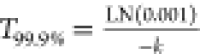ula , in the case of the simple exponential model, where k is the decay rate constant. In the case of the biphasic model, we used the formula 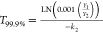, where Y₁ and Y₂ are concentrations corresponding to the intercepts of each phase of the biphasic model and k₂ is the decay rate constant for the second phase. This 1000-fold decrease in initial eDNA concentrations reflects the approximate decrease from the eDNA starting concentration to the LOQ or LOD typical of eDNA persistence studies and is thus ecologically and methodologically relevant.

Results and Discussion

Modeling eDNA Degradation

eDNA degradation did not show a trend consistent with a simple exponential decay process in our experiments. Instead, it showed a general trend of decreasing degradation rate over time. The simple exponential model consistently underestimated measured eDNA concentrations at earlier time points and overestimated them at intermediate time points (Figure S2). Lower BIC and significant likelihood ratio tests indicated that the biphasic model better fit the data from 20 of the 22 experiments (Table S1). We report the results of the biphasic model for the two experiments in which the biphasic model did not have a significantly better fit because the slopes of the initial and second phases were similar. The biphasic model’s average breakpoint, parameter b, was 38.9 ± 18.6 h (Table S2). In all experiments, the decay rate constant was greater during the initial phase (steeper slope) than during the second phase (Figure 2).

A decreasing rate of eDNA degradation may be explained by a decrease in the size of particles that the eDNA is associated with over time.²⁰⁻²² Field and experimental studies show that eDNA is present primarily in relatively large size fractions, between 1 and 10 μm, including whole cells and mitochondria.^58,63,64 Experimental work indicates that the proportion of eDNA in large-size fractions decreases rapidly. However, the proportion of eDNA in size fractions smaller than 3 μm increases over time, and its degradation is slower than the degradation of eDNA in larger size fractions.^20,21 Our observations indicating that the degradation rate decreased over time may reflect a shift in the association of eDNA with larger particles (e.g., cells or organelles) to smaller particles.²⁰⁻²²

Since tissue homogenization and freezing likely lysed Lophelia cells, most of the eDNA early on in our experiments may not have been exclusively contained within cells but likely included free DNA or DNA in mitochondria. We assume that it is unlikely that eDNA was adsorbed to foreign particulates in our experiments because we used filtered artificial seawater. It seems likely that free DNA would pass through the 0.22 μm non-polar filter membrane we used. However, a recent study found that a 0.45 μm non-charged membrane can recover measurable concentrations free DNA molecules from seawater.⁶⁵ In our experiments, the observed rapid initial decrease of eDNA may be explained not only by the degradation of DNA in mitochondria but also by the lysis of mitochondria and the loss of free DNA that passes through the filter. Persistent, low concentrations of eDNA at later time points may reflect remaining whole mitochondria, free DNA captured on the filter, or free DNA associated with material from the Lophelia tissue.

In addition to spawning, it is likely that eDNA from corals is also shed through mucus production. Lophelia maintains a protective mucus layer, sheds mucus in response to disturbance, and may also produce mucus nets as a strategy to capture prey.^66,67 Previous studies have quantified eDNA shedding for Lophelia and two species of hydrozoans.^8,32,59 However, the state of eDNA that Lophelia and other cnidarians shed through processes such as mucus secretion remains unknown. Experiments that concurrently quantify coral eDNA shedding and mucus secretion would be informative, especially if the state of shed eDNA is determined.

Effects of Temperature, pH, and Oxygen Concentration on eDNA Degradation

Temperature

Our findings support the hypothesis that temperature is the most significant controlling factor of eDNA degradation rate in seawater. The effect of temperature was substantial in the second phase of eDNA degradation but not in the initial phase. During the initial phase of eDNA degradation, the estimated decay rate constants among experiments conducted at 20 °C (mean ± SD = 0.084 ± 0.016 h^–1) were, on average, higher than those conducted at 10 °C (0.070 ± 0.014 h^–1) and 4 °C (0.073 ± 0.013 h^–1; Figure 3A). However, there was no significant effect of any predictor variable when fitting an LMM to the initial phase dataset (Table S3). Therefore, we find no evidence that eDNA degradation is influenced by temperature, pH, or [DO] early in the experiments before the model breakpoint.

Figure 3.

Decay rate constant (k) estimates for the initial (A) and second (B) phases of eDNA degradation for 22 experiments conducted across 11 combinations of temperature, pH, and [DO]. Decay rate constants were estimated by fitting an exponential decay equation with initial and second degradation phases with different rates (biphasic). Decay rate constants are arranged on the x axis by the average pH over the course of each experiment. Vertical error bars represent 95% confidence intervals for the decay rate constants. The color of each point represents the average [DO] over each experiment.

Second phase decay rate constants in experiments conducted at 20 °C (0.036 ± 0.017 h^–1) were substantially higher than those at 10 °C (0.011 ± 0.002 h^–1) and 4 °C (0.018 ± 0.004 h^–1; Figure 3B). In the second phase, the interaction between temperature and time (in days) was the most significant predictor of eDNA concentration (P = 0.003; Table S4). Consistently, the interaction between temperature and time was the only significant predictor (P = 0.035) of eDNA concentration among the subset of pH 8.2 experiments conducted at 4 and 20 °C (Table S5). In addition, the effect size for the interaction of temperature and time was greater than the effect size for any other model term (Tables S4 and S5). These results imply that the temperature and time since the addition of eDNA are the strongest predictors of eDNA concentration in our experiments. We interpret that temperature controls the persistence of eDNA more strongly than pH or [DO].

The fact that temperature strongly controlled eDNA persistence only during the second phase of the experiments suggests that this effect may depend on the eDNA state. As stated previously, we propose that faster degradation during the initial phase of our experiments may reflect the lysis of mitochondria. Degradation of eDNA in smaller size fractions may be dominant in the second phase. If this is the case, our results contrast with a recent meta-analysis that found that the effect of temperature on eDNA degradation rate is stronger in studies using filter pore sizes of >0.7 μm than pore sizes of <0.45 μm.²² Our results suggest that the persistence of eDNA in smaller size fractions may have been more affected by temperature than the persistence in larger size fractions.

pH

Our findings tentatively support the hypothesis that pH may influence the eDNA degradation rate in seawater. In the second phase, pH was a marginally significant predictor of eDNA concentration (P = 0.048; Table S4). The effect size of pH was substantially smaller than the effect size of the interaction between time and temperature (Table S4). The LMM fit to the subset of the second-phase data that excluded experiments conducted at 20 °C indicated that the interaction of time and pH is a nearly significant predictor of eDNA concentration (P = 0.069; Table S6). Indeed, higher pH among experiments conducted at 4 °C was associated with higher decay rate constants (Pearson’s r = 0.601, P = 0.039; Figure 3B). We infer from these results that pH may affect the persistence of eDNA in the range of marine conditions that we tested. However, this effect is small compared to that of temperature.

Previous work in freshwater systems has demonstrated that eDNA degrades faster at more acidic pH values. Lance et al. investigated a pH range similar to our study’s (7.5 and 8.0)^27,29,37,38 and found that lower pH was associated with faster eDNA degradation in freshwater.²⁹ Here, we present data suggesting that relatively more acidic seawater with a pH near 7.6 may prolong the persistence of eDNA compared to seawater at higher pH. Our results suggest that the influence of pH on eDNA degradation in seawater may need to be further considered.

Dissolved Oxygen Concentration

Our findings do not support the hypothesis that [DO] is a significant controlling factor of eDNA degradation in seawater. We conducted experiments in a fully factorial design with a full range of [DO] at two temperatures (4 and 20 °C) and a pH of 8.2. In the LMMs fit to this subset of the data and the full second-phase dataset, neither average [DO], average ORP, nor the interaction of these factors with time were significant predictors of eDNA concentration (Tables S4 and S5). From these results, we infer that [DO] and the oxidative state of seawater have the least influence on eDNA degradation rate and persistence among the conditions we tested. Thus, eDNA degradation may be driven by oxygen-independent processes.

Temperature Dependence of eDNA Degradation in the Marine Environment

Environmental DNA persistence times estimated from our study are comparable to previous marine studies performed at similar temperatures regardless of the source species (Figure 4). For example, eDNA persistence times from a skate at 4 °C (T_99.9% = 14.4 and 26.2 days)²³ fall within our calculated persistence times for Lophelia (T_99.9% range = 12.5 to 28.8 days). Further, persistence times from our experiments at 10 °C (T_99.9% range = 16.0 to 24.0 days) are comparable to the persistence time calculated using data from a previous study of Lophelia eDNA degradation using natural seawater and live coral at 8 °C (T_99.9% = 16.9 days).⁸

Figure 4.

eDNA persistence time (time until degradation of 99.9% of starting eDNA concentration), estimated using decay rate constants from our study and other published marine studies, as a function of temperature. The linear model was only fit to decay rate constants calculated from simple exponential models. The best fit line is indicated by the dashed line, and the shaded region represents the 95% confidence interval for the slope. Points are dodged slightly from actual recorded temperatures to improve visualization. (Inset) Comparison of calculated persistence times when fitting a single exponential versus a biphasic model to the data in this study. Data are reported in Table S7.

We fit a linear model to eDNA persistence time (time until degradation of 99.9% of starting eDNA concentration), estimated using decay rate constants from our study and other published marine studies, and temperature (Figure 4). We found that this model has a satisfactory fit (adjusted R² = 0.4792, P < 0.001). The model predicts that eDNA persistence decreases by ∼0.74 days for each increase in degrees Celsius. Our results align with findings by Allan et al. They demonstrated a positive linear relationship between temperature and decay rate constants in most studies investigating eDNA degradation at multiple temperatures.³² Similarly, Mauvisseau et al. found a linear relationship between increased temperature and faster decay rate constant in studies of freshwater and marine fish.¹² Further investigations at intermediate (∼8 to 12 °C) and high temperatures (greater than ∼25 °C), as well as more studies of invertebrate taxa, would improve confidence in the generality of this model. This model does not consider other factors that may influence eDNA quantification or detection in the ocean, including microbial activity, pH, advection, or diffusion. However, it serves as a resource to approximate maximum eDNA persistence times, constrained by temperature, in the marine environment.

Implications for eDNA Quantification and Sequencing in the Marine Environment

Investigating the spatiotemporal scale of eDNA in the marine environment is critical to defining the spatiotemporal resolution of ecological information derived from eDNA quantification or detection. Recent studies have found that eDNA abundance can exhibit strong vertical stratification, from just 5 m below the surface to 2000 m deep in the mesopelagic open ocean and within the first 10 m below the surface in nearshore habitats.^47,68,69 Further, model simulations have suggested that eDNA in the ocean remains within tens of meters from the depth where it is shed.⁷⁰ Field data from eDNA sampling along short, horizontal transects has revealed discrete eDNA community profiles at a fine scale in diverse shallow-water habitats, including coral reefs and kelp forests.^6,71,72 Together, these results suggest that eDNA community profiles, obtained using techniques such as meta-barcoding, can accurately reflect biological communities structured by depth. However, the ability of eDNA meta-barcoding to distinguish communities in deep-sea environments is less clear. eDNA sequencing efforts in the deep sea have resulted in benthic community composition profiles that agree with expected differences due to habitat at sites ∼15 km apart.⁷³ However, eDNA sampling paired with video analyses revealed remarkable disparities between video observations and sequence read abundances from deep-sea corals.⁷ Some coral species were observed in video surveys but were not detected in eDNA, and many sequence reads were recovered from species not observed in videos.

Modeling studies suggest that the extent of horizontal transport of eDNA at concentrations detectable through single-species quantitative methods can be substantial, on the order of tens of kilometers, in the surface ocean and at depth.^8,26 These models provide valuable insights for understanding the horizontal spatial scale of eDNA in the ocean. However, studies modeling eDNA transport have utilized decay rate constants derived from simple exponential models.^8,26 We found that at low temperatures of ≤10 °C, a simple exponential model can substantially underestimate the persistence of eDNA. Environmental DNA persistence time, defined as the time until degradation of 99.9% of the starting eDNA concentration, was up to 75% longer when fitting the data with the biphasic model rather than the simple exponential model (Figure 4 and Table S7). Thus, in cold marine environments including the deep sea, detectable eDNA may be transported over longer distances than predicted by simulations that assumed a simple exponential decay.

The interpretation of field eDNA data from deep-sea corals is complicated because eDNA may persist for longer durations at cold temperatures and may be shed infrequently or at low concentrations. We conducted field sampling within 1 m of a large aggregation of live Lophelia and at altitudes of 5, 10, and 20 m above the seafloor in the Gulf of Mexico. We found that caryophylliid eDNA could be detected (positive qPCR amplification) within 10 m above the seafloor. However, copy number estimates were below the LOQ of our qPCR assay (Table S8; see the Supplementary Methods). Kutti et al. also measured relatively low concentrations of Lophelia eDNA in the Norwegian Sea (up to 1000 s of copies per L of seawater filtered), demonstrating that Lophelia eDNA is present at low concentrations in its environment.⁸

If eDNA in nature is shed at low concentrations, it may be diluted rapidly and degrade past the detectable limit more quickly than in an experimental setting. Thus, an eDNA sample may provide an accurate signal of the proximate biological community. However, our experiments demonstrate that eDNA can persist for weeks at low temperatures, so detectable concentrations may be transported over large distances. When using single-species quantitative methods, such as qPCR or digital-droplet PCR, considerable care should be taken when interpreting the source of a positive eDNA amplification. We suggest that a range of possible sources must be considered for an observed eDNA signal. This range can be constrained by coupling estimated persistence times and hydrodynamic models.

Supporting Information Available

The Supporting Information is available free of charge at https://pubs.acs.org/doi/10.1021/acs.est.2c01672.

• Supplementary methods; supplementary figures and tables referenced in the main text; supplementary table supporting qPCR inhibition testing as described in the Supplementary Methods (PDF)

This research was funded by the National Oceanic and Atmospheric Administration’s Oceanic and Atmospheric Research, Office of Ocean Exploration and Research, under award NA18OAR0110289 to S.H. and J.M.M. at Lehigh University, and sub-awards to E.E.C at Temple University and C.S.M. at Harvey Mudd College.

The authors declare no competing financial interest.

Notes

All data and R-code are available at 10.6084/m9.figshare.19775608.

References

- Barnosky A. D.; Matzke N.; Tomiya S.; Wogan G. O. U.; Swartz B.; Quental T. B.; Marshall C.; McGuire J. L.; Lindsey E. L.; Maguire K. C.; Mersey B.; Ferrer E. A. Has the Earth’s Sixth Mass Extinction Already Arrived?. Nature 2011, 471, 51–57. 10.1038/nature09678. [DOI] [PubMed] [Google Scholar]
- Dirzo R.; Young H. S.; Galetti M.; Ceballos G.; Isaac N. J. B.; Collen B. Defaunation in the Anthropocene. Science 2014, 345, 401–406. 10.1126/science.1251817. [DOI] [PubMed] [Google Scholar]
- McCauley D. J.; Pinsky M. L.; Palumbi S. R.; Estes J. A.; Joyce F. H.; Warner R. R. Marine Defaunation: Animal Loss in the Global Ocean. Science 2015, 347, 1255641. 10.1126/science.1255641. [DOI] [PubMed] [Google Scholar]
- Thomsen P. F.; Willerslev E. Environmental DNA - An Emerging Tool in Conservation for Monitoring Past and Present Biodiversity. Biol. Conserv. 2015, 183, 4–18. 10.1016/j.biocon.2014.11.019. [DOI] [Google Scholar]
- Breed M. F.; Harrison P. A.; Blyth C.; Byrne M.; Gaget V.; Gellie N. J. C.; Groom S. V. C.; Hodgson R.; Mills J. G.; Prowse T. A. A.; Steane D. A.; Mohr J. J. The Potential of Genomics for Restoring Ecosystems and Biodiversity. Nat. Rev. Genet. 2019, 20, 615–628. 10.1038/s41576-019-0152-0. [DOI] [PubMed] [Google Scholar]
- Port J. A.; O’Donnell J. L.; Romero-Maraccini O. C.; Leary P. R.; Litvin S. Y.; Nickols K. J.; Yamahara K. M.; Kelly R. P. Assessing Vertebrate Biodiversity in a Kelp Forest Ecosystem Using Environmental DNA. Mol. Ecol. 2016, 25, 527–541. 10.1111/mec.13481. [DOI] [PMC free article] [PubMed] [Google Scholar]
- Everett M. V.; Park L. K. Exploring Deep-Water Coral Communities Using Environmental DNA. Deep Sea Res., Part II 2018, 150, 229–241. 10.1016/j.dsr2.2017.09.008. [DOI] [Google Scholar]
- Kutti T.; Johnsen I. A.; Skaar K. S.; Ray J. L.; Husa V.; Dahlgren T. G. Quantification of eDNA to Map the Distribution of Cold-Water Coral Reefs. Front. Mar. Sci. 2020, 7, 1–12. 10.3389/fmars.2020.00446.32802822 [DOI] [Google Scholar]
- Whitaker J. M.; Brower A. L.; Janosik A. M. Invasive Lionfish Detected in Estuaries in the Northern Gulf of Mexico Using Environmental DNA. Environ. Biol. Fishes 2021, 104, 1475–1485. 10.1007/s10641-021-01177-6. [DOI] [Google Scholar]
- Keller A. G.; Grason E. W.; McDonald P. S.; Ramón-Laca A.; Kelly R. P. Tracking an Invasion Front with Environmental DNA. Ecol. Appl. 2022, e2561 10.1002/eap.2561. [DOI] [PubMed] [Google Scholar]
- Barnes M. A.; Turner C. R. The Ecology of Environmental DNA and Implications for Conservation Genetics. Conserv. Genet. 2016, 17, 1–17. 10.1007/s10592-015-0775-4. [DOI] [Google Scholar]
- Mauvisseau Q.; Harper L. R.; Sander M.; Hanner R. H.; Kleyer H.; Deiner K. The Multiple States of Environmental DNA and What Is Known about Their Persistence in Aquatic Environments. Environ. Sci. Technol. 2022, 5322. 10.1021/acs.est.1c07638. [DOI] [PMC free article] [PubMed] [Google Scholar]
- Maruyama A.; Nakamura K.; Yamanaka H.; Kondoh M.; Minamoto T. The Release Rate of Environmental DNA from Juvenile and Adult Fish. PLoS One 2014, 9, e114639 10.1371/journal.pone.0114639. [DOI] [PMC free article] [PubMed] [Google Scholar]
- Klymus K. E.; Richter C. A.; Chapman D. C.; Paukert C. Quantification of eDNA Shedding Rates from Invasive Bighead Carp Hypophthalmichthys nobilis and Silver Carp Hypophthalmichthys molitrix. Biol. Conserv. 2015, 183, 77–84. 10.1016/j.biocon.2014.11.020. [DOI] [Google Scholar]
- Lacoursière-Roussel A.; Côté G.; Leclerc V.; Bernatchez L. Quantifying Relative Fish Abundance with EDNA: A Promising Tool for Fisheries Management. J. Appl. Ecol. 2016, 53, 1148–1157. 10.1111/1365-2664.12598. [DOI] [Google Scholar]
- Sansom B. J.; Sassoubre L. M. Environmental DNA (eDNA) Shedding and Decay Rates to Model Freshwater Mussel EDNA Transport in a River. Environ. Sci. Technol. 2017, 51, 14244–14253. 10.1021/acs.est.7b05199. [DOI] [PubMed] [Google Scholar]
- Jo T.; Arimoto M.; Murakami H.; Masuda R.; Minamoto T. Estimating Shedding and Decay Rates of Environmental Nuclear DNA with Relation to Water Temperature and Biomass. Environ. DNA 2020, 2, 140–151. 10.1002/edn3.51. [DOI] [Google Scholar]
- Ostberg C. O.; Chase D. M. Ontogeny of eDNA Shedding during Early Development in Chinook Salmon (Oncorhynchus tshawytscha). Environ. DNA 2022, 339. 10.1002/edn3.258. [DOI] [Google Scholar]
- Thalinger B.; Rieder A.; Teuffenbach A.; Pütz Y.; Schwerte T.; Wanzenböck J.; Traugott M. The Effect of Activity, Energy Use, and Species Identity on Environmental DNA Shedding of Freshwater Fish. Front. Ecol. Evol. 2021, 9, 1–13. 10.3389/fevo.2021.623718. [DOI] [Google Scholar]
- Jo T.; Arimoto M.; Murakami H.; Masuda R.; Minamoto T. Particle Size Distribution of Environmental DNA from the Nuclei of Marine Fish. Environ. Sci. Technol. 2019, 53, 9947–9956. 10.1021/acs.est.9b02833. [DOI] [PubMed] [Google Scholar]
- Jo T.; Murakami H.; Yamamoto S.; Masuda R.; Minamoto T. Effect of Water Temperature and Fish Biomass on Environmental DNA Shedding, Degradation, and Size Distribution. Ecol. Evol. 2019, 9, 1135–1146. 10.1002/ece3.4802. [DOI] [PMC free article] [PubMed] [Google Scholar]
- Jo T.; Minamoto T. Complex Interactions between Environmental DNA (eDNA) State and Water Chemistries on eDNA Persistence Suggested by Meta-analyses. Mol. Ecol. Resour. 2021, 21, 1490–1503. 10.1111/1755-0998.13354. [DOI] [PubMed] [Google Scholar]
- Weltz K.; Lyle J. M.; Ovenden J.; Morgan J. A. T.; Moreno D. A.; Semmens J. M. Application of Environmental DNA to Detect an Endangered Marine Skate Species in the Wild. PLoS One 2017, 12, e0178124 10.1371/journal.pone.0178124. [DOI] [PMC free article] [PubMed] [Google Scholar]
- Collins R. A.; Wangensteen O. S.; O’Gorman E. J.; Mariani S.; Sims D. W.; Genner M. J. Persistence of Environmental DNA in Marine Systems. Commun. Biol. 2018, 1, 1–11. 10.1038/s42003-018-0192-6. [DOI] [PMC free article] [PubMed] [Google Scholar]
- Harrison J. B.; Sunday J. M.; Rogers S. M. Predicting the Fate of eDNA in the Environment and Implications for Studying Biodiversity. Proc. R. Soc. B 2019, 286, 20191409. 10.1098/rspb.2019.1409. [DOI] [PMC free article] [PubMed] [Google Scholar]
- Andruszkiewicz E. A.; Koseff J. R.; Fringer O. B.; Ouellette N. T.; Lowe A. B.; Edwards C. A.; Boehm A. B. Modeling Environmental DNA Transport in the Coastal Ocean Using Lagrangian Particle Tracking. Front. Mar. Sci. 2019, 6, 1–14. 10.3389/fmars.2019.00477. [DOI] [Google Scholar]
- Strickler K. M.; Fremier A. K.; Goldberg C. S. Quantifying Effects of UV-B, Temperature, and pH on eDNA Degradation in Aquatic Microcosms. Biol. Conserv. 2015, 183, 85–92. 10.1016/j.biocon.2014.11.038. [DOI] [Google Scholar]
- Eichmiller J. J.; Best S. E.; Sorensen P. W. Effects of Temperature and Trophic State on Degradation of Environmental DNA in Lake Water. Environ. Sci. Technol. 2016, 50, 1859–1867. 10.1021/acs.est.5b05672. [DOI] [PubMed] [Google Scholar]
- Lance R.; Klymus K.; Richter C.; Guan X.; Farrington H.; Carr M.; Thompson N.; Chapman D.; Baerwaldt K. Experimental Observations on the Decay of Environmental DNA from Bighead and Silver Carps. MBI 2017, 8, 343–359. 10.3391/mbi.2017.8.3.08. [DOI] [Google Scholar]
- Tsuji S.; Ushio M.; Sakurai S.; Minamoto T.; Yamanaka H. Water Temperature-Dependent Degradation of Environmental DNA and Its Relation to Bacterial Abundance. PLoS One 2017, 12, 1–13. 10.1371/journal.pone.0176608. [DOI] [PMC free article] [PubMed] [Google Scholar]
- Kasai A.; Takada S.; Yamazaki A.; Masuda R.; Yamanaka H. The Effect of Temperature on Environmental DNA Degradation of Japanese Eel. Fish. Sci. 2020, 86, 465–471. 10.1007/s12562-020-01409-1. [DOI] [Google Scholar]
- Allan E. A.; Zhang W. G.; Lavery A. C.; Govindarajan A. F. Environmental DNA Shedding and Decay Rates from Diverse Animal Forms and Thermal Regimes. Environ. DNA 2021, 3, 492–514. 10.1002/edn3.141. [DOI] [Google Scholar]
- Caza-Allard I.; Laporte M.; Côté G.; April J.; Bernatchez L. Effect of Biotic and Abiotic Factors on the Production and Degradation of Fish Environmental DNA: An Experimental Evaluation. Environ. DNA 2022, 4, 453–468. 10.1002/edn3.266. [DOI] [Google Scholar]
- Lindahl T.; Nyberg B. Rate of Depurination of Native Deoxyribonucleic Acid. Biochemistry 1972, 11, 3610–3618. 10.1021/bi00769a018. [DOI] [PubMed] [Google Scholar]
- Cheng Y.-K.; Pettitt B. M. Stabilities of Double- and Triple-Strand Helical Nucleic Acids. Prog. Biophys. Mol. Biol. 1992, 58, 225–257. 10.1016/0079-6107(92)90007-s. [DOI] [PubMed] [Google Scholar]
- Lindahl T. Instability and Decay of the Primary Structure of DNA. Nature 1993, 362, 709–715. 10.1038/362709a0. [DOI] [PubMed] [Google Scholar]
- Seymour M.; Durance I.; Cosby B. J.; Ransom-Jones E.; Deiner K.; Ormerod S. J.; Colbourne J. K.; Wilgar G.; Carvalho G. R.; de Bruyn M.; Edwards F.; Emmett B. A.; Bik H. M.; Creer S. Acidity Promotes Degradation of Multi-Species Environmental DNA in Lotic Mesocosms. Commun. Biol. 2018, 1, 1–8. 10.1038/s42003-017-0005-3. [DOI] [PMC free article] [PubMed] [Google Scholar]
- van Bochove K.; Bakker F. T.; Beentjes K. K.; Hemerik L.; Vos R. A.; Gravendeel B. Organic Matter Reduces the Amount of Detectable Environmental DNA in Freshwater. Ecol. Evol. 2020, 10, 3647–3654. 10.1002/ece3.6123. [DOI] [PMC free article] [PubMed] [Google Scholar]
- Lalli C. M.; Parsons T. R.. Biological Oceanography: An Introduction; Elsevier: (Second Edition). 1997. [Google Scholar]
- Paulmier A.; Ruiz-Pino D. Oxygen Minimum Zones (OMZs) in the Modern Ocean. Prog. Oceanogr. 2009, 80, 113–128. 10.1016/j.pocean.2008.08.001. [DOI] [Google Scholar]
- Addamo A. M.; Vertino A.; Stolarski J.; García-Jiménez R.; Taviani M.; Machordom A. Merging Scleractinian Genera: The Overwhelming Genetic Similarity between Solitary Desmophyllum and Colonial Lophelia. BMC Evol. Biol. 2016, 16, 108. 10.1186/s12862-016-0654-8. [DOI] [PMC free article] [PubMed] [Google Scholar]
- Cordes E. E.; McGinley M. P.; Podowski E. L.; Becker E. L.; Lessard-Pilon S.; Viada S. T.; Fisher C. R. Coral Communities of the Deep Gulf of Mexico. Deep Sea Res., Part I 2008, 55, 777–787. 10.1016/j.dsr.2008.03.005. [DOI] [Google Scholar]
- Lessard-Pilon S. A.; Podowski E. L.; Cordes E. E.; Fisher C. R. Megafauna Community Composition Associated with Lophelia pertusa Colonies in the Gulf of Mexico. Deep Sea Res., Part II 2010, 57, 1882–1890. 10.1016/j.dsr2.2010.05.013. [DOI] [Google Scholar]
- Andruszkiewicz E. A.; Sassoubre L. M.; Boehm A. B. Persistence of Marine Fish Environmental DNA and the Influence of Sunlight. PLoS One 2017, 12, e0185043 10.1371/journal.pone.0185043. [DOI] [PMC free article] [PubMed] [Google Scholar]
- Tedetti M.; Sempéré R. Penetration of Ultraviolet Radiation in the Marine Environment. A Review. Photochem. Photobiol. 2006, 82, 389–397. 10.1562/2005-11-09-ir-733. [DOI] [PubMed] [Google Scholar]
- Spens J.; Evans A. R.; Halfmaerten D.; Knudsen S. W.; Sengupta M. E.; Mak S. S. T.; Sigsgaard E. E.; Hellström M. Comparison of capture and storage methods for aqueous macrobial eDNA using an optimized extraction protocol: advantage of enclosed filter. Methods Ecol. Evol. 2017, 8, 635–645. 10.1111/2041-210x.12683. [DOI] [Google Scholar]
- Govindarajan A. F.; Francolini R. D.; Jech J. M.; Lavery A. C.; Llopiz J. K.; Wiebe P. H.; Zhang W. G. Exploring the Use of Environmental DNA (eDNA) to Detect Animal Taxa in the Mesopelagic Zone. Front. Ecol. Evol. 2021, 9, 1–17. 10.3389/fevo.2021.574877. [DOI] [Google Scholar]
- Klymus K. E.; Merkes C. M.; Allison M. J.; Goldberg C. S.; Helbing C. C.; Hunter M. E.; Jackson C. A.; Lance R. F.; Mangan A. M.; Monroe E. M.; Piaggio A. J.; Stokdyk J. P.; Wilson C. C.; Richter C. A. Reporting the Limits of Detection and Quantification for Environmental DNA Assays. Environ. DNA 2020, 2, 271–282. 10.1002/edn3.29. [DOI] [Google Scholar]
- Wickham H.Ggplot2: Elegant Graphics for Data Analysis; Springer-Verlag: New York, 2016. [Google Scholar]
- Shogren A. J.; Tank J. L.; Egan S. P.; August O.; Rosi E. J.; Hanrahan B. R.; Renshaw M. A.; Gantz C. A.; Bolster D. Water Flow and Biofilm Cover Influence Environmental DNA Detection in Recirculating Streams. Environ. Sci. Technol. 2018, 52, 8530–8537. 10.1021/acs.est.8b01822. [DOI] [PubMed] [Google Scholar]
- Bylemans J.; Furlan E. M.; Gleeson D. M.; Hardy C. M.; Duncan R. P. Does Size Matter? An Experimental Evaluation of the Relative Abundance and Decay Rates of Aquatic Environmental DNA. Environ. Sci. Technol. 2018, 52, 6408–6416. 10.1021/acs.est.8b01071. [DOI] [PubMed] [Google Scholar]
- Muggeo V. M. R. Estimating Regression Models with Unknown Break-points. Stat. Med. 2003, 22, 3055–3071. 10.1002/sim.1545. [DOI] [PubMed] [Google Scholar]
- Bates D.; Mächler M.; Bolker B.; Walker S. Fitting Linear Mixed-Effects Models Using Lme4. J. Stat. Softw. 2015, 67, 1–48. 10.18637/jss.v067.i01. [DOI] [Google Scholar]
- Kuznetsova A.; Brockhoff P. B.; Christensen R. H. B. LmerTest Package: Tests in Linear Mixed Effects Models. J. Stat. Softw. 2017, 82, 1–26. 10.18637/jss.v082.i13. [DOI] [Google Scholar]
- Ben-Shachar M.; Lüdecke D.; Makowski D. Effectsize: Estimation of Effect Size Indices and Standardized Parameters. J. Open Source Softw. 2020, 5, 2815. 10.21105/joss.02815. [DOI] [Google Scholar]
- Harrison X. A.; Donaldson L.; Correa-Cano M. E.; Evans J.; Fisher D. N.; Goodwin C. E. D.; Robinson B. S.; Hodgson D. J.; Inger R. A Brief Introduction to Mixed Effects Modelling and Multi-Model Inference in Ecology. Peerj 2018, 6, e4794 10.7717/peerj.4794. [DOI] [PMC free article] [PubMed] [Google Scholar]
- Thomsen P. F.; Kielgast J.; Iversen L. L.; Møller P. R.; Rasmussen M.; Willerslev E. Detection of a Diverse Marine Fish Fauna Using Environmental DNA from Seawater Samples. PLoS One 2012, 7, e41732 10.1371/journal.pone.0041732. [DOI] [PMC free article] [PubMed] [Google Scholar]
- Sassoubre L. M.; Yamahara K. M.; Gardner L. D.; Block B. A.; Boehm A. B. Quantification of Environmental DNA (eDNA) Shedding and Decay Rates for Three Marine Fish. Environ. Sci. Technol. 2016, 50, 10456–10464. 10.1021/acs.est.6b03114. [DOI] [PubMed] [Google Scholar]
- Minamoto T.; Fukuda M.; Katsuhara K. R.; Fujiwara A.; Hidaka S.; Yamamoto S.; Takahashi K.; Masuda R. Environmental DNA Reflects Spatial and Temporal Jellyfish Distribution. PLoS One 2017, 12, e0173073 10.1371/journal.pone.0173073. [DOI] [PMC free article] [PubMed] [Google Scholar]
- Wood S. A.; Biessy L.; Latchford J. L.; Zaiko A.; von Ammon U.; Audrezet F.; Cristescu M. E.; Pochon X. Release and Degradation of Environmental DNA and RNA in a Marine System. Sci. Total Environ. 2020, 704, 135314 10.1016/j.scitotenv.2019.135314. [DOI] [PubMed] [Google Scholar]
- Kwong S. L. T.; Villacorta-Rath C.; Doyle J.; Uthicke S. Quantifying Shedding and Degradation Rates of Environmental DNA (eDNA) from Pacific Crown-of-Thorns Seastar (Acanthaster cf. solaris). Mar. Biol. 2021, 168, 1–10. 10.1007/s00227-021-03896-x. [DOI] [Google Scholar]
- Kirtane A.; Wieczorek D.; Noji T.; Baskin L.; Ober C.; Plosica R.; Chenoweth A.; Lynch K.; Sassoubre L. Quantification of Environmental DNA (eDNA) Shedding and Decay Rates for Three Commercially Harvested Fish Species and Comparison between EDNA Detection and Trawl Catches. Environ. DNA 2021, 3, 1142–1155. 10.1002/edn3.236. [DOI] [Google Scholar]
- Turner C. R.; Barnes M. A.; Xu C. C. Y.; Jones S. E.; Jerde C. L.; Lodge D. M. Particle size distribution and optimal capture of aqueous macrobial eDNA. Methods Ecol. Evol. 2014, 5, 676–684. 10.1111/2041-210x.12206. [DOI] [Google Scholar]
- Wilcox T. M.; McKelvey K. S.; Young M. K.; Lowe W. H.; Schwartz M. K. Environmental DNA Particle Size Distribution from Brook Trout (Salvelinus fontinalis). Conserv. Genet. Resour. 2015, 7, 639–641. 10.1007/s12686-015-0465-z. [DOI] [Google Scholar]
- Zaiko A.; von Ammon U.; Stuart J.; Smith K. F.; Yao R.; Welsh M.; Pochon X.; Bowers H. A. Assessing the Performance and Efficiency of Environmental DNA/RNA Capture Methodologies under Controlled Experimental Conditions. Methods Ecol. Evol. 2022, 10.1111/2041-210x.13879. [DOI] [Google Scholar]
- Bythell J. C.; Wild C. Biology and Ecology of Coral Mucus Release. J. Exp. Mar. Biol. Ecol. 2011, 408, 88–93. 10.1016/j.jembe.2011.07.028. [DOI] [Google Scholar]
- Murray F.; De Clippele L. H.; Hiley A.; Wicks L.; Roberts J. M.; Hennige S. Multiple Feeding Strategies Observed in the Cold-Water Coral Lophelia pertusa. J. Mar. Biol. Assoc. U. K. 2019, 99, 1281–1283. 10.1017/s0025315419000298. [DOI] [Google Scholar]
- Canals O.; Mendibil I.; Santos M.; Irigoien X.; Rodríguez-Ezpeleta N. Vertical Stratification of Environmental DNA in the Open Ocean Captures Ecological Patterns and Behavior of Deep-sea Fishes. Limnol. Oceanogr. Lett. 2021, 6, 339–347. 10.1002/lol2.10213. [DOI] [Google Scholar]
- Monuki K.; Barber P. H.; Gold Z. eDNA Captures Depth Partitioning in a Kelp Forest Ecosystem. PLoS One 2021, 16, e0253104 10.1371/journal.pone.0253104. [DOI] [PMC free article] [PubMed] [Google Scholar]
- Allan E. A.; DiBenedetto M. H.; Lavery A. C.; Govindarajan A. F.; Zhang W. G. Modeling Characterization of the Vertical and Temporal Variability of Environmental DNA in the Mesopelagic Ocean. Sci. Rep. 2021, 11, 21273. 10.1038/s41598-021-00288-5. [DOI] [PMC free article] [PubMed] [Google Scholar]
- West K. M.; Stat M.; Harvey E. S.; Skepper C. L.; DiBattista J. D.; Richards Z. T.; Travers M. J.; Newman S. J.; Bunce M. eDNA Metabarcoding Survey Reveals Fine-Scale Coral Reef Community Variation across a Remote, Tropical Island Ecosystem. Mol. Ecol. 2020, 29, 1069–1086. 10.1111/mec.15382. [DOI] [PubMed] [Google Scholar]
- Lamy T.; Pitz K. J.; Chavez F. P.; Yorke C. E.; Miller R. J. Environmental DNA Reveals the Fine-Grained and Hierarchical Spatial Structure of Kelp Forest Fish Communities. Sci. Rep. 2021, 11, 1–13. 10.1038/s41598-021-93859-5. [DOI] [PMC free article] [PubMed] [Google Scholar]
- Laroche O.; Kersten O.; Smith C. R.; Goetze E. Environmental DNA Surveys Detect Distinct Metazoan Communities across Abyssal Plains and Seamounts in the Western Clarion Clipperton Zone. Mol. Ecol. 2020, 29, 4588–4604. 10.1111/mec.15484. [DOI] [PMC free article] [PubMed] [Google Scholar]
Associated Data
This section collects any data citations, data availability statements, or supplementary materials included in this article.