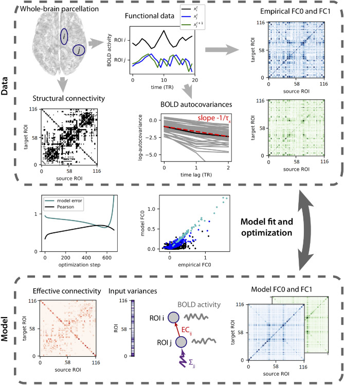
Fig. 1.

Model parameters estimation (adapted from Gilson et al. 2020). To capture BOLD dynamics, the model uses the time-series parcellated into 116 ROIs (box on the left top) to calculate two autocovariance matrices (FC0 and FC1 matrices) both with and without time lag (blue and green lines in the central box on top). The SC connectivity matrix (black and white matrix on the left) is used as a binary matrix to constrain the model’s topology to existing connections. Besides the effective connectivity estimates (Pink matrix at the left bottom), the autocovariance matrices (green and blue matrices at the right bottom) are also reproduced by the dynamic model. The model undergoes an optimization procedure so that, at each step, the estimated FC matrices are evaluated with regards to the empirical FC0 and FC1 matrices. The optimization steps are repeated until reaching a high Pearson correlation coefficient between the model’s and the empirical FC matrices, reducing this way the model error (depicted as the green and black lines in the central box on the left of the figure)