Figure 6.

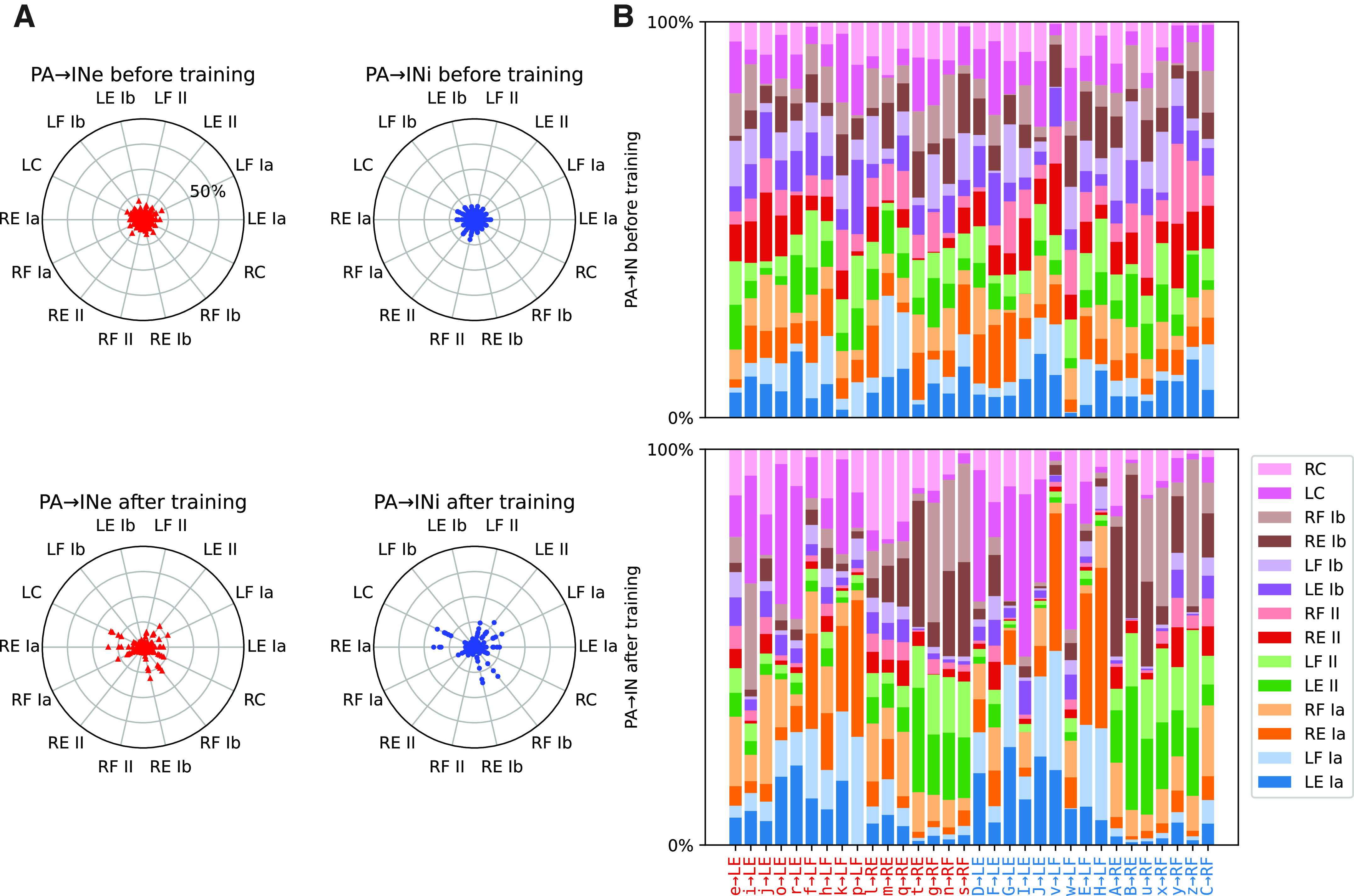
Training-induced development of primary afferent input connectivity in the interneurons in the example simulation. State before training is shown in the top row, whereas the bottom row shows the state after 400,000 s of training. A: the synaptic weight for each primary afferent relative to the total synaptic weight of the primary afferents. Radial plots for excitatory interneurons (INe, left) and inhibitory interneurons (INi, right) before (top) and after (bottom) training. Similar pairs of proprioceptive sensors are on opposite sides of the circle. The initial homogenous spread is replaced with a heterogeneous specialization with training. B: stacked bar chart of the relative primary afferent synaptic weight distribution before (top) and after (bottom) training. The interneurons have the same order as in Fig. 5., i.e., ordered according to their strongest efferent projection onto the β motoneurons (βMNs). Once again it can be seen that the initially random relative strengths give way to specificity for both sensory modality and limb origin. LE, left extensor; LF, left flexor; PA, primary afferent; RE, right extensor; RF, right flexor.