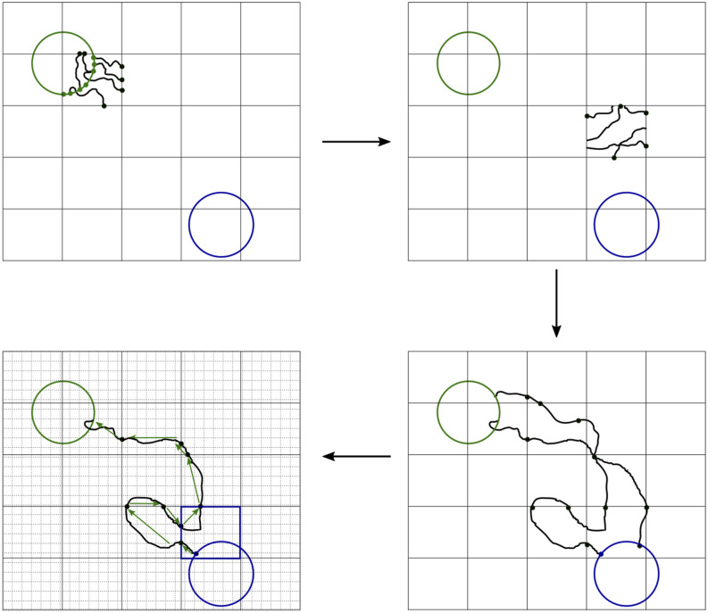
FIG. 1.
Schematic of the algorithm. (upper left) Define the metastable states and the strata (black grid) and initialize the data structures (step 1). In the example shown, trajectories are initialized from the upper left metastable state boundary, so the last metastable state visited is known. (upper right) In each stratum, draw configurations from γij(dx), save pointers to the associated γij(dx) elements, and then run unbiased dynamics from these configurations until the trajectories exit the stratum (steps 2b and 2c). A single example stratum is shown. (lower right) As the simulation progresses, each point in γij(dx) may give rise to segments of reactive or unreactive trajectories. Save the collective variable values associated with these trajectory segments (step 2d). (lower left) When a reactive or unreactive trajectory is realized (i.e., a trajectory segment enters a metastable state), trace back from pointer to pointer to determine the sequences of strata and collective variable grid sites (gray grid) visited (step 3). Use these to increment unnormalized statistics with appropriate weights (steps 3a–3c). Note that the collective variable grid sites and the strata need not coincide.

