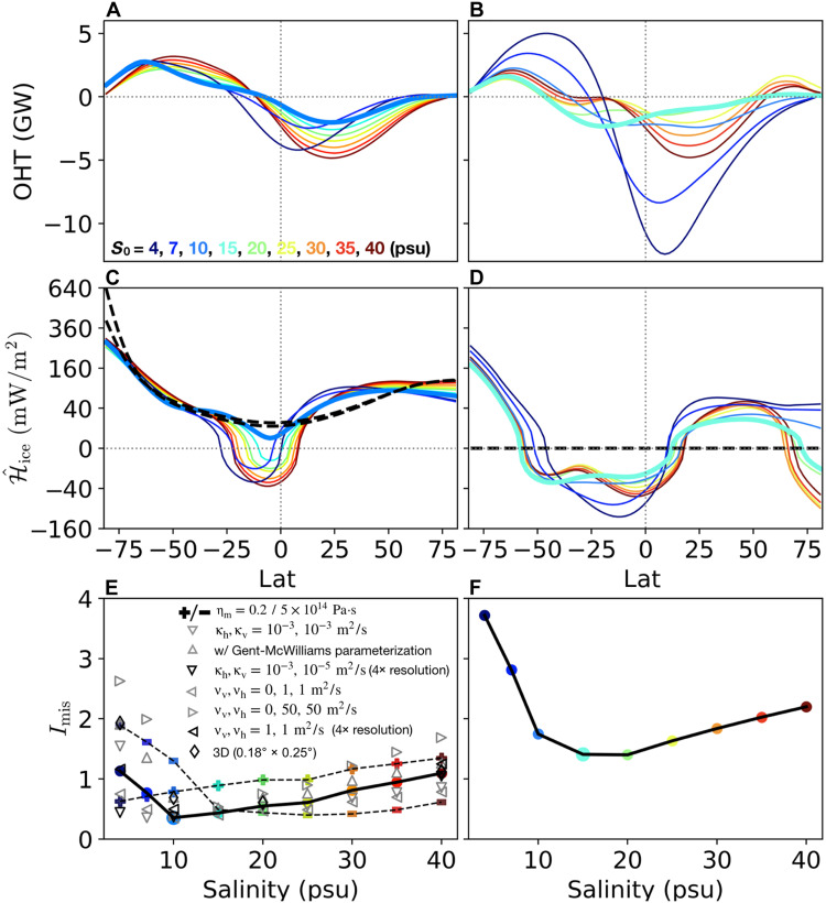
Fig. 4. Meridional heat transport and heat budget.

Left column shows the shell-heating scenario and the right column shows the core-heating scenario. The top panels (A and B) show the vertically integrated meridional OHT for various assumed S₀. Positive values denote northward heat transport. The middle panels (C and D) show the inferred tidal heating ${\widehat{\mathscr{H}}}_{\text{ice}}$ (solid curves), in comparison with the heating predicted by a tide model ℋ_ice (dashed curves). As a measure of uncertainties in the tide model, two p_α values, −2 and −1, are used to compute ℋ_ice. The black dashed curves in (D) coincide with the zero line, because ℋ_ice = 0 when all heating is in the core. The bottom panels (E and F) show the mismatch index I_mis, defined in Eq. 3. Filled colored dots connected by a thick solid line correspond to the default setup (horizontal/vertical diffusivity κ_h= κ_v = 0.005 m²/s, horizontal/vertical viscosity ν_h = ν_v = 10 m²/s, 100% heat produced in the ice, and melting-point ice viscosity η_m = 10¹⁴ Pa·s). Other symbols represent sensitivity tests to ice viscosity, mixing coefficients, and model resolution. The I_mix of the low and high η_m experiments are multiplied by a factor of 0.3 and 2, respectively, so that all plots make use of the same scale.