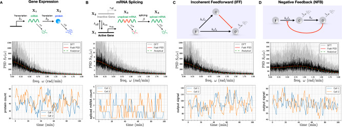
Fig. 2. Frequency-domain analysis of linear propensity networks.

A This is the standard gene expression model where mRNA (X₁) is transcribed constitutively and it translates into protein (X₂). B In this RNA splicing network a gene can randomly switch between inactive (X₂) (low transcription) and active (X₁) (high transcription) states. When transcription occurs, unspliced mRNA (X₃) is created which is then converted into spliced mRNA (X₄) by the splicing machinery. C In the Incoherent Feedforward (IFF) network an input I (constant level I₀) directly produces the output O and it produces the controller species C, which represses the production of output O. D In the Negative Feedback (NFB) network the input I (constant level I₀) produces the controller species C, that produces the output species O which in turn inhibits the production of C from I. For all the networks single-cell output trajectories in the stationary phase are plotted. We provide a comparison of the single-cell PSDs estimated with three approaches—(1) analytically (see Table 1), (2) the Padé PSD method (see Table 1) using Q = 10 simulated trajectories and (3) the averaged periodogram or the DFT method mentioned in Box 1 using discrete samples from Q = 10 simulated trajectories. For the DFT estimator, the black curve represents the mean of the PSDs and the shaded grey region represents the symmetric one standard deviation interval around the mean. For the NFB network one can see that detecting the presence of oscillations in the fluctuations is much easier in the frequency-domain than in the time-domain.