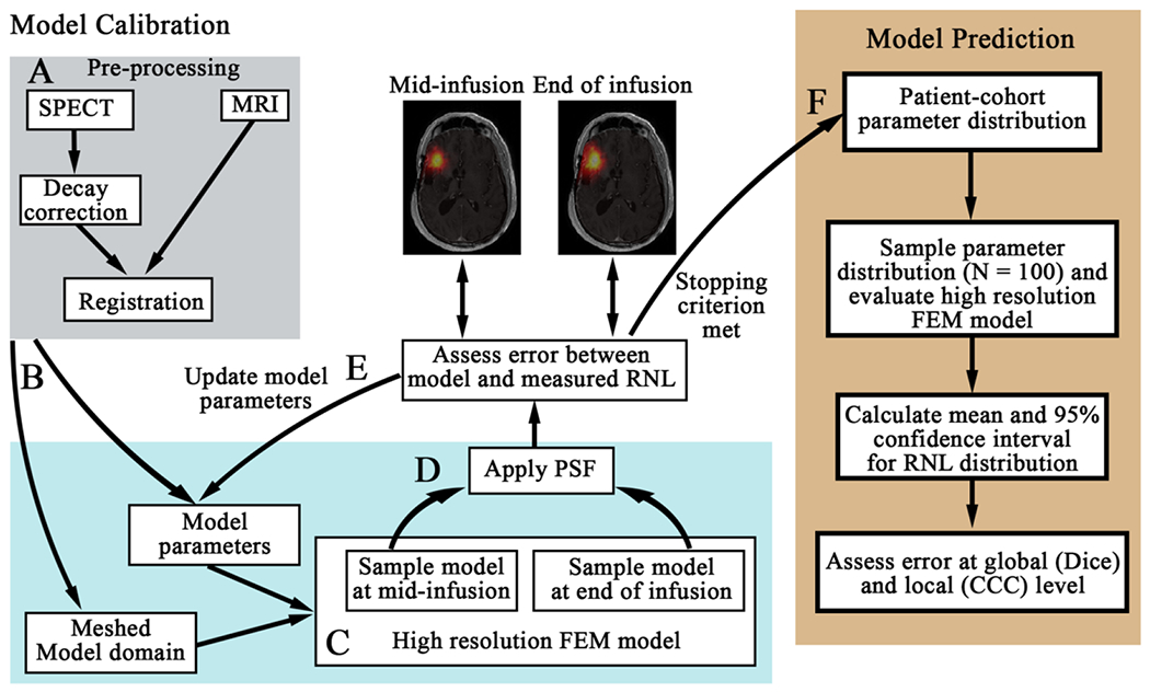
Figure 1. Schematic of the patient-specific modeling framework.

First, the SPECT data is decay corrected and co-registered to the MRI data (panel A). The registered domains are used to generate the FEM mesh (arrow B) and assign spatially-varying model parameters. Each model within the model family is then run forward using an initial guess of model parameters on the high-resolution mesh (panel C). The model estimated distribution of RNL is sampled at the mid-infusion and end of infusion time points. We apply our estimated point spread function (PSF) of the SPECT data and resample the image to the lower-resolution of the SPECT data (arrow D). The error between the model estimated distribution of RNL and the measured distribution are compared. Model parameters are updated (arrow E) until stopping criterion are met (arrow F). The optimized model parameters are saved for the patient-cohort parameter distribution (arrow F). Once all of the models are calibrated for each patient, we then performed our prediction scenario using a leave-one-out approach (right panel). We first determine the cohort parameter distribution using data from all but the patient whose RNL distribution we will predict. We sample this distribution 100 times and evaluate the high-resolution FEM model. The mean and 95% confidence interval are calculated from the 100 simulations, and the mean predicted RNL distribution is compared to the measured RNL distribution at the global and local levels.