Fig. 5.
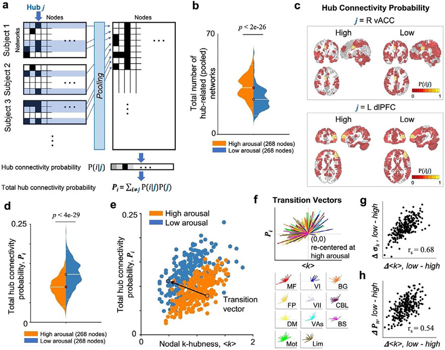
Resting state networks at low arousal have reduced network overlaps while exhibiting brain-wide connectivity. (a) A summary diagram to calculate hub connectivity probability (pi = P(i∣j)) and total hub connectivity probability (Pi). For an arousal state, resting state networks involving a hub j are collected from all subjects. pi: the conditional probability of each node i to be a member of functional networks overlapping in a hub j. (b) The total number of hub-related networks for each node is lower at low relative to high arousal. (c) Probability maps of functional connectivity integrated in a specific hub (two exemplary nodes in the right vACC and the left dlPFC) across subjects. (d) Pi is higher at low relative to high arousal across the whole brain, indicating an increased global synchronization. (e) Scatter plot of hub measures from 268 nodes at high (orange) and low (blue) arousal data. X-axis denotes the group average k-hubness (<k>). Y-axis denotes Pi calculated for each node i. Left (L)/Right (R) in bold. An exemplary transition vector that links a node at high arousal state (<k>high, Pi(high)) to the same node at low arousal state (<k>low, Pi(low)) is shown. (f) Re-centered transition vectors for all nodes, from (0,0) to (<k>low- <k>high, Pi(low)- Pi(high)), show a trend pointing toward the quadrant II, indicating a decrease in k-hubness and an increase in Pi from high to low arousal. Transition vectors for nodes in each large-scale network (color-coded as in Figs. 2-4) are shown below. Nodes exhibiting large group-average changes in <k> also exhibit large changes in inter-subject variability (g) and total connectivity probability (h) (rs: Spearman’s rank correlation, p=0).

