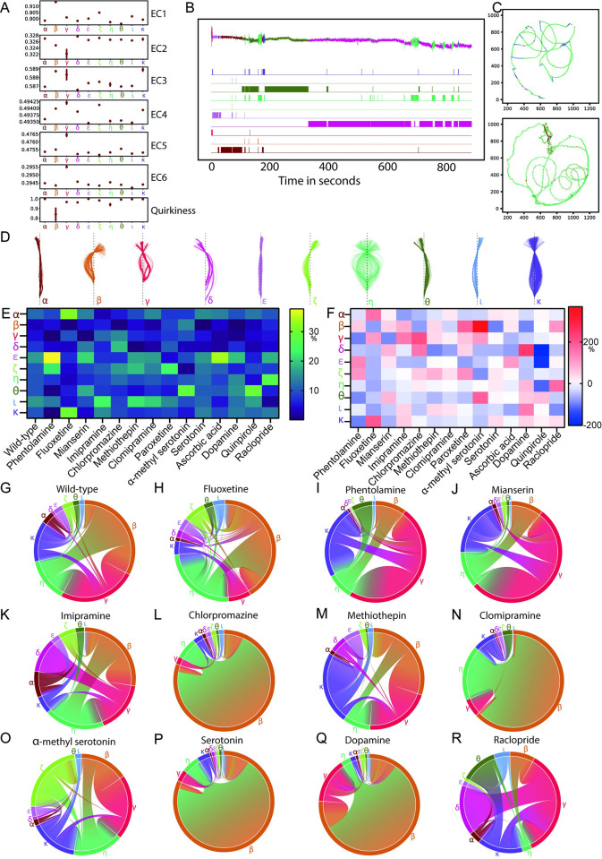
Fig 4. HMM analysis reveals that behavioral transitions in Ciona are modulated by bioamines.
(A) Plots summarizing the observation probability distributions defined by the HMM model. For each of the states (horizontal axes), the mean of Gaussian distributions of each of the 7 input features is plotted along the vertical axes. The variance of the distributions is indicated by the error bars (underlying data can be found in S20–S22 Tables and https://doi.org/10.5281/zenodo.6761771). (B) HMM segments and clusters a time series into modules by identifying the underlying state for each time point in the series. On the top, eigencoefficient EC1 (a time series) of a larva swimming is annotated with the different HMM states (uniquely color coded) identified in our analysis. (C) Two example tracks of the neck point of larvae in the arena colored according to the behavioral state identified by HMM. (D) Postures/skeletons were randomly sampled 90 skeletons from the dataset for each of the 10 different HMM states, aligned such that the neck points coincide and are collinear with tail-ends on a vertical line. (E) Heatmap visualization of the effects of drug treatments on the HMM-derived behavioral states (values in % can be found in S23 Table). (F) Heatmap visualization of percentage fold changes relative to wild type for the data shown in panel E (values in % can be found in S24 Table). Dopamine values are compared relative to ascorbic acid and not wild type. Drugs that resulted in a statistically significant up-regulation or down-regulation of the usage of HMM states are listed in S56 Table. (G–R) Chord diagrams showing HMM-derived behavioral state transitions for wild type and drug-treated larvae. Chord diagrams are presented in such a way that transition to all other states with probabilities greater than 0.001 are shown. Underlying data can be obtained from https://doi.org/10.5281/zenodo.6761771. EC1, Eigenciona 1; EC2, Eigenciona 2; EC3, Eigenciona 3; EC4, Eigenciona 4; EC5, Eigenciona 5; EC6, Eigenciona 6; HMM, hidden Markov model.

