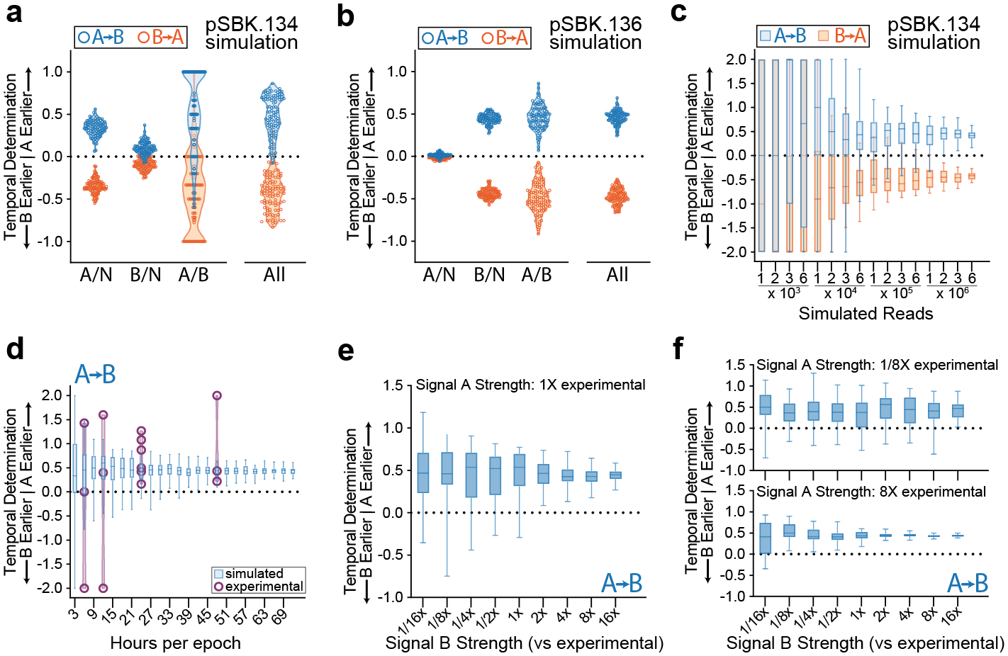
Figure 5. Modeling the Limits of Retron Recording.

a. Simulation of 100 replicates each of A-then-B and B-then-A recordings using acquisition rate data from pSBK.134 recordings. Each point represents the calculated ordering score from a single replicate of 1 million arrays. b. Simulation of 100 replicates each of A-then-B and B-then-A recordings using acquisition rate data from pSBK.136 recordings. Each point represents the calculated ordering score from a single replicate of 1 million arrays. c. Simulation of varying the number of arrays analyzed per sample using acquisition rate data from pSBK.134 recordings. Each box with whiskers represents 100 simulated replicates, with whiskers extending from minimum to maximum. d. Simulation of varying the length of each epoch in a retron recording using acquisition rate data from pSBK.134 (blue). Overlaid with real retron recordings of the same length (purple). Each box with whiskers represents 100 simulated replicates of 1 million reads each, with whiskers spanning from minimum to maximum. Each overlaid point is a single biological replicate. Recording experiments with 6, 12, and 48-hour epochs were done in triplicate. Recording experiments with epoch length of 24 hours are the same as in Figure 4l. e. Simulation of varying the strength of signal B when signal A remains constant. 1x acquisition rates were obtained from pSBK.134 recordings. Each box with whiskers represents 50 simulated replicates of 1 million arrays each. Whiskers span from minimum to maximum. f. Simulation of varying the strength of signal B when signal A is decreased or increased by a factor of 8. 1x acquisition rates were obtained from pSBK.134 recordings. Each box with whiskers represents 50 simulated replicates of 1 million arrays each. Whiskers span from minimum to maximum.