Harmonized neonatal brain MR image segmentation model for cross-site datasets

Abstract

Accurate segmentation of white matter, gray matter and cerebrospinal fluid from neonatal brain MR images is of great importance in characterizing early brain development. Deep-learning-based methods have been successfully applied to neonatal brain MRIs with superior performance if testing subjects were acquired with the same imaging protocols/scanners as training subjects. However, for the testing subjects acquired with different imaging protocols/scanners, they cannot achieve accurate segmentation results due to large appearance/pattern differences between the testing and training subjects. Besides, imaging artifacts, like head motion, which are inevitable during the imaging acquisition process, also pose a challenge for the segmentation methods. To address these issues, in this paper, we propose a harmonized neonatal brain MR image segmentation model that harmonizes testing images acquired by different protocols/scanners into the domain of training images through a cycle-consistent generative adversarial network (CycleGAN). Meanwhile, the artifacts can be largely alleviated during the harmonization. Then, a densely-connected U-Net based segmentation model trained in the domain of training images can be applied robustly for segmenting the harmonized testing images. Comparisons with existing methods illustrate the better performance of the proposed method on neonatal brain MR images from cross-sites, a grand segmentation challenge, as well as images with artifacts.

1. Introduction

Accurate segmentation of white matter (WM), gray matter (GM), and cerebrospinal fluid (CSF) from neonatal brain MR images is an important prerequisite for characterizing early postnatal brain growth and development [1]. Compared with manual segmentation, automated segmentation is time-saving and not prone to inter- and intra-observer variability. Therefore, accurate and automated segmentation methods are highly needed. However, neonatal brain MR images typically exhibit reduced tissue contrast, large within-tissue intensity variations, and regionally-heterogeneous dynamic image appearance and development, in comparison with adult brain MR images [2].

Many computational methods, especially deep-learning-based methods (e.g., U-Net [3], X-Net [4], CLCI-Net [5], D-UNet [6]), have been successfully applied to medical image analysis, including neonatal brain MR image segmentation. For example, Zhang et al. designed four convolutional neural network (CNN) architectures to segment infant brain tissues based on multimodal MR images, where each CNN contained three input feature maps corresponding to T1w, T2w, and fractional anisotropy (FA) image patches [7]. Nie et al. proposed to use multiple fully convolutional networks (FCNs) to segment isointense-phase brain images with T1w, T2w, and FA modality information [8]. Some more advanced deep-learning-based methods have also been reported in the iSeg-2017 challenge review article [9].

Although these methods have achieved encouraging results, there are still several limitations: (1) deep-learning-based methods can achieve superior performance when the testing subjects are acquired with the same imaging protocol/scanner as the training images, but degraded performance when the testing subjects are acquired with different imaging protocols/scanners as the training images [10]. This is known as the multi-site issue or domain-shift issue [11]. For example, Fig. 1 presents two neonatal images acquired with different imaging protocols. It can be seen from the zoomed views that tissue intensities/appearances in Fig. 1(a) are different from those in Fig. 1(b), e.g., Fig. 1(b) is smoother than Fig. 1(a). These differences may degrade the performance of the trained deep-learning-based models. (2) neonatal brain images are often corrupted with imaging artifacts like motions during image acquisition [2], as shown in Fig. 2.

Fig. 1.

Comparison between two T1-weighted MR images from the source domain (a) and the target domain (b). These images were acquired with different parameters and scanners, as listed in Table 1. (c) shows the harmonized image of (b) with a more consistent appearance with (a), compared to (b).

Fig. 2.

A neonatal MR image with motion artifacts.

To address these problems, one feasible way is to use domain adaptation methods [12], by which we can transfer knowledge learned from a source domain with labels, to a target domain without labels [11]. Most domain adaption methods are supervised-based, either finding a mapping between the source domain and the target domain [13] or identifying domain-invariant representations that are shared between two domains [14,15]. For example, Sadda et al. presented a method for the generation of synthetic examples using cyclic generative adversarial neural networks for retinal vessel segmentation [16]. Huo et al. proposed an end-to-end synthetic segmentation network (SynSeg-Net) to train a segmentation network for a target imaging modality without manual labels [17,18]. Khalili et al. proposed the method using the same procedure with the 2D version of CycleGAN [19]. Dewey et al. also proposed a deep-learning approach for contrast harmonization across scanners to improve the segmentation performance [20]. Dong et al. proposed an unsupervised domain adaptation framework for chest organ segmentation based on adversarial networks [21]. Wang et al. proposed a segmentation network in which multi-level feature space and output space adversarial learning were leveraged to transfer discriminative domain knowledge across different datasets for multi-sequence cardiac MR images [22]. Kuling et al. presented a breast segmentation pipeline that uses multiple U-Net segmentation models trained on different image types [23]. Aiming at learning segmentation without ground truth in target modality, Zhou et al. proposed an anatomy-preserving domain adaptation to segmentation network for intraprocedural CBCT/MR liver segmentation [24]. However, the previous works either need the paired images [20], or were proposed for multimodal scenarios, such as between MRI and CT [17,18], or only focus on a single dataset [19], or only work on 2D images [16–24]. Few works are focusing on the segmentation of 3D neonatal brain MR images from cross-site datasets.

In this work, we propose a harmonized neonatal brain MR image segmentation model for cross-site dataset scenarios, in which manual labels are only available for training subjects in the source domain. Specifically, we first train a densely-connected U-Net (DcU-Net for short) to segment the neonatal brain MR images in the source domain. Then, given any testing image from the target domain, we employ the 3D CycleGAN to harmonize each testing image to the source domain (shown in Fig. 1(c)). Finally, the trained segmentation model is applied to the harmonized testing image for tissue segmentation. In such a way, the segmentation model trained in the source domain can be directly applied to any new datasets by the proposed harmonization.

The main contributions of our work are summarized as follows:

1. We propose a general harmonization framework for neonatal brain MR image segmentation which can handle the testing subjects from multiple sites with different imaging protocols/scanners.

2. The proposed work is robust to the imaging artifacts.

3. The proposed method can also handle subjects with different ages.

The remainder of this paper is organized as follows. Section 2 introduces the dataset and preprocessing procedures. Section 3 illuminates the framework of the harmonized segmentation model and details on every single component. The experimental results are presented in Section 4, followed by discussions and conclusion in Section 5.

2. Dataset and image preprocessing

The source dataset consists of 30 neonatal T1-weighted MR images, from Multi-visit Advanced Pediatric (MAP) Brain Imaging Study, acquired on a Siemens head-only 3T scanners, with 144 sagittal slices, TR/TE = 1900/4.38 ms, and resolution = 1.0 × 1.0 × 1.0 mm³. The target dataset consists of 40 T1-weighted neonatal MR images, from Xi’an Jiaotong University (XJU), acquired on a GE 3T scanner, with 120 slices, TR/TE = 10.47/4.76 ms, and resolution = 0.9 × 0.9 × 1.0 mm³. The details of two datasets are shown in Table 1.

Table 1.

Parameters of data acquisition for the source and target datasets.

Datasets	Age	Scanner	TR (ms)	TE (ms)	Resolution (mm3)
Source: MAP	0-month	Siemens 3T	1900	4.38	1.0 × 1.0 × 1.0
Target: XJU	0-month	GE 3T	10.47	4.76	0.9 × 0.9 × 1.0

Before tissue segmentation, we resampled all images into the same resolution of 1.0 × 1.0 × 1.0 mm³, and then performed skull stripping, intensity inhomogeneity correction [25], as well as cerebellum and brain stem removal. Five images were randomly selected from the source dataset for label annotation and used as the training samples to train the segmentation network.

3. Method

Fig. 3 illustrates the framework of the proposed method, which is called harmonized densely-connected U-Net (HDcU-Net for short) and consists of two training stages and one testing stage. The source domain (S for short) is provided with paired intensity images and manual labels, while the target domain (T for short) is provided with only intensity images from any other site. We firstly train segmentation model based on the paired intensity images and manual labels in source domain via DcU-Net, and then leverage 3D CycleGAN to train a generator network for the harmonization between source and target domains. Finally, in the testing stage, trained harmonization and segmentation models are applied to testing subjects from the target domain.

Fig. 3.

Illustration of the proposed harmonized neonatal brain MR image segmentation method. The top-left part and top-right part show the 3D tissue segmentation network and the 3D CycleGAN in the training stage. The lower part shows the testing stage for images in the target domain, which needs a trained generator G₁ (T → S) for harmonizing each testing image in the target domain to the source domain and also a trained segmentation network for tissue segmentation.

3.1. Training of the segmentation network

Training of the tissue segmentation module is illustrated in the top-left part of Fig. 3. Many network architectures can be used to train the segmentation model. In this paper, we adopt a recently proposed DcU-Net as the segmentation network (shown in Fig. 4), which has achieved superior performance for isointense (at around 6-month-old of age) infant brain segmentation [26]. The DcU-Net includes an encoder path and a decoder path, going through seven dense blocks. In the encoder path, between any two contiguous dense blocks, a transition down block is included to reduce the feature map resolution and increase the receptive field. While in the decoder path, a transition up block, consisting of a transposed convolution, is included between any two contiguous dense blocks. It up-samples the feature maps from the preceding dense block. The up-sampled feature maps are then concatenated with those coming from the skip connection to form the input for the posterior dense block. Each dense block consists of three BN-ReLU-Conv-Dropout operations, in which each Conv includes 16 kernels and the dropout rate is 0.1. For all the convolutional layers, the kernel size is 3 × 3 × 3 with stride size 1 and 0-padding. The loss function is cross-entropy in the network, which is represented as L_Seg in Fig. 3. For the training dataset, we first flipped the original images in axial view as data augmentation to double the number of training subjects. Then, we randomly extracted 3D patches with a size of 32 × 32 × 32 from training images. Specifically, a total of 6000 patches are extracted for each subject. During the training, we set the learning rate as 0.01 with step decreasing, gamma as 0.1, momentum as 0.9, and weight decay as 0.0005.

Fig. 4.

Diagram of the architecture of the DcU-Net.

3.2. Harmonization through CycleGAN

Harmonization procedure is implemented through the 3D CycleGAN, as illustrated in the top-right part of Fig. 3. G₁ and G₂ are two generators for learning the mappings from T to S and from S to T, respectively. D₁ and D₂ are two discriminators for determining whether the input image is real or not for S and T, respectively. Adversarial losses are adopted for both mapping functions in CycleGAN, and the discrimination loss can be written as [27]:

$$\begin{gathered} L_{\text{GAN}}=E_{y~S}\left[\log D_1(y)\right]+E_{x~T}\left[\log \left(1-D_1\left(G_1(x)\right)\right)\right]+E_{x~T}\left[\log D_2(x)\right] \\ +E_{y~S}\left[\log \left(1-D_2\left(G_2(y)\right)\right)\right] \end{gathered}$$ (1)

where G tries to generate images G(x) that look similar to images from domain T, while D aims to distinguish between translated samples G(x) and real samples y. G aims to minimize this objective against an adversary D that tries to maximize it.

Meanwhile, the cycle-consistent loss is also proposed to ensure the mapped images into any domain can be mapped back to the original domain. As shown in Fig. 3, for each image x from domain S, the image translation cycle should be able to bring x back to the original images, i. e. x→G₁(x)→G₂(G₁(x))≈x. The cycle consistency loss can be described as [27]:

$$L_{\text{Cycle}}=E_{y~S}\left[{\Vert G_1\left(G_2(y)\right)-y\Vert }_1\right]+E_{x~T}\left[{\Vert G_2\left(G_1(x)\right)-x\Vert }_1\right]$$ (2)

The overall loss function for the CycleGAN is:

$$L=L_{\text{GAN}}+\lambda L_{\text{Cycle}}$$ (3)

3D convolution kernels are applied in the convolution layers of generators and discriminators. For the generators and discriminators, ResNet [28] with three residual blocks and the fully convolutional network with five convolutional layers are adopted respectively. 3D patches are randomly extracted from 3D images as inputs to the generators and the discriminators to avoid overload of GPU memory usage. The size of the patch is 32 × 32 × 32. Note that patches with only background information are excluded. We set the learning rate as 0.0002, λ as 10, and momentum as 0.5.

3.3. Testing of CycleGAN and segmentation

In the testing stage, the original images from the target domain are harmonized into the source domain via the trained CycleGAN. Then, the harmonized images are segmented into different tissue types by the trained DcU-Net in the source domain, as illustrated in Fig. 3. Although we could also alternatively harmonize training images from source domain into each target domain (each site) using G₂, we will have to train a segmentation model for each site. By contrast, our strategy only needs to train one single segmentation model for all cross-sites.

4. Experimental results

To validate the proposed method, we first demonstrated the effectiveness on cross-site datasets with the same age, including the robustness of our method against motion artifacts. We then validated our method on the MICCAI Grand Challenge of Neonatal Brain Segmentation 2012 (NeoBrainS12) [29]. Furthermore, we demonstrated the effectiveness on cross-site datasets with different ages. For evaluation, the manual segmentation is considered as the “ground truth” for comparison.

4.1. Evaluation metrics

We mainly employed Dice coefficient (DC) for the segmentation accuracy evaluation, which is defined as:

$$\text{DC}=2|A\cap B|/(|A|+|B|)$$ (4)

where A and B represent manual and automatic segmentation results of the same image, respectively.

We also employed the modified Hausdorff distance (MHD) to evaluate the segmentation accuracy, which is defined as the 95th-percentile Hausdorff distance:

$$\text{MHD}(A,B)=\max {(}^{95}{K}_{\alpha \in \text{surf}(A)}^{\text{th}}d\left(\alpha ,\text{surf}(B){,}^{95}{K}_{\beta \in \text{surf}(B)}^{\text{th}}d(\beta ,\text{surf}(A))\right)$$ (5)

where surf(A) is the surface of segmentation A, $K_{\alpha \in \text{surf}(A)}^{\text{th}}$ represents the K^th ranked distance such that K/|surf(A)| = 95%, and d(α, surf(B) is the nearest Euclidean distance from a surface point α to the surface B.

4.2. Results on cross-site datasets

To train the segmentation network DcU-Net, we employed 5 images with manual annotations from the source domain (MAP, shown in Table 1). To train the 3D CycleGAN, we used 20 T1w images without manual labels from MAP and 20 T1w images without manual labels from the target domain (XJU, shown in Table 1). The source images from MAP are free of artifact and the CycleGAN loss will make appearance patterns of target images to be similar with the source images. Training/testing were performed on a NVIDIA Titan X GPU. Basically, training a DcU-Net and CycleGAN took around 48 h and 60 h respectively and segmenting a 3D image by the proposed strategy required 180–200 s totally in the testing stage. Specifically, time-consuming of harmonization procedure took 110–120 s and segmenting procedure took 70–80 s.

For comparison, we trained two models using a U-Net [3] and the DcU-Net in the source domain and then applied them to the target domain, with two presentative results shown in the first two rows of Fig. 5. Due to the multi-site issue or domain-shift issue, the trained models cannot generalize well, with CSF and GM incorrectly identified as WM, as indicated by the dashed contour. It is worth noting that the input images for the U-Net and the DcU-Net were preprocessed by histogram matching with the source domain before applying the segmentation models. By contrast, with the proposed harmonization, the harmonized target images and their corresponding results are shown in the third row and fourth row of Fig. 5, respectively. We can see that both segmentation results of the U-Net and the DcU-Net are greatly improved, especially in the region indicated by the dashed contour, demonstrating the effectiveness of the proposed harmonization for the neonatal brain segmentation from cross-sites.

Fig. 5.

Comparisons of results without/with the harmonization on a neonatal MR image in the target domain. The first row shows the target image from XJU and segmentation result obtained by the U-Net, and the second row shows the segmentation result obtained by the DcU-Net. The third row shows the harmonized target image and their corresponding segmentation result by the harmonized U-Net, and the fourth row shows the segmentation result by HDcU-Net (the proposed method). The fifth row shows the manual segmentation.

For a quantitative comparison, the average DC and MHD evaluated on 8 subjects from XJU with manual labels are presented in Table 2, which shows that the proposed strategy achieves higher DC and lower MHD values in tissue segmentation for different networks (shown in the gray shade of Table 2). We further test the statistical significance between different results and find that the proposed method has a strongly statistically significant difference on WM/DC compared with the U-Net (p-value = 0.002) and harmonized U-Net (p-value = 0.017), and a weak statistical significance compared with the DcU-Net (p-value = 0.035).

Table 2.

Averaged Dice coefficient (in percentage) and MHD (in mm) for different methods for tissue segmentation of 8 neonatal brain MR images in cross-site scenario.

Method	Tissue	U-Net	Harmonized U-Net	DcU-Net	H DcU-Net (the proposed)
DC	WM	90.89±2.12	93.23±0.68	91.93±2.40	93.79±0.67
	GM	83.94±1.76	85.50±0.84	85.22±2.30	86.95±0.60
	CSF	83.38±1.62	84.38±1.24	86.54±2.30	87.35±0.96
MHD (in mm)	WM	1.43±0.29	0.99±0.14	1.19±0.33	0.95±0.02
	GM	1.13±0.18	1.29±0.61	1.10±0.27	1.08±0.37
	CSF	3.12±0.43	2.11±0.33	2.83±0.61	1.89±0.26

4.3. Robust to the artifacts

To demonstrate the robustness in the presence of artifacts, we added simulated motion artifacts via Gibbs effect onto the motion-free intensity images and made comparisons between segmentations results on the motion-free and motion-corrupted images. As shown in Fig. 6, the first and the second rows respectively present segmentation results by the DcU-Net and HDcU-Net on a motion-free neonatal brain MR image. The simulated motion-corrupted image is shown in the third row. Then we applied the DcU-Net and HDcU-Net to this motion corrupted image, with results shown in the third and fourth rows. It can be found that the DcU-Net cannot perform well in the presence of motion artifacts with many segmentation errors in the 3D surrendering result, compared with the segmentation in the first row without the motion artifacts. While using the proposed harmonization, the motion artifacts are largely alleviated, and the segmentation performance is greatly improved (the fourth row).

Fig. 6.

Comparisons of results without/with harmonization for neonatal MR image without/with motion artifacts in the target domain. The first row shows the target image from XJU and the corresponding segmentation result by DcU-Net. The second row shows the harmonized image and corresponding segmentation result by HDcU-Net (the proposed method). The third row shows the image with motion artifacts and the corresponding segmentation result by the DcU-Net. The fourth row shows the harmonized image and corresponding segmentation result by HDcU-Net. The fifth row shows the manual segmentation.

For a quantitative comparison, we evaluated 8 images from XJU with simulated motion artifacts. The average DC and MHD for the results on the motion-free and motion-corrupted images by the methods without/with harmonization are presented in Table 3. It can be found that the proposed method achieves a higher Dice coefficient and lower MHD values than the DcU-Net, on both the motion-free and motion-corrupted images (shown in the gray shade of Table 3). We also calculated the p-values, in terms of {WM, GM, CSF}/DC, using the paired-sample t-tests to show the statistical significance among methods. After adding motion artifacts, the DcU-Net (the fifth column) has lower DC values in terms of WM, GM and CSF segmentations, as well as a strong statistical difference compared with those without motion artifacts (the third column) (WM: p-value = 0.009, GM: p-value = 0.008), which demonstrate that the DcU-Net is sensitive to motion artifacts. However, the results of the proposed HDcU-Net method (the last column) are similar with those results without motion artifacts (the fourth column), and there is only weak statistical difference in terms of WM (WM: p-value = 0.032) and no statistical difference in terms of GM and CSF (GM: p-value = 0.161, CSF: p-value = 0.989), which indicate the proposed method is robust to motion artifacts.

Table 3.

Averaged Dice coefficient (in percentage) and MHD (in mm) for different methods for tissue segmentation of 8 neonatal MR images without/with motion artifacts in the target domain.

Method	Tissue	Without motion artifacts		With motion artifacts
		DcU-Net	HDcU-Net	DcU-Net	HDcU-Net
			(the proposed)		(the proposed)
DC	WM	91.93±2.40	93.79±0.67	90.57±2.72	93.08±1.06
	GM	85.22±2.30	86.95±0.60	83.91±2.54	87.22±0.77
	CSF	86.54±2.30	87.35±0.96	85.69±2.86	87.36±0.93
MHD (in mm)	WM	1.19±0.33	0.95±0.02	1.28±0.48	1.25±0.51
	GM	1.10±0.27	1.08±0.37	1.17±0.36	0.99±0.14
	CSF	2.83±0.61	1.89±0.26	2.47±0.43	1.73±0.22

4.4. Results on the NeobrainS12 MICCAI challenge

We further validated our method on NeoBrainS12 MICCAI challenge (http://neobrains12.isi.uu.nl) [29]. In the challenge, two preterm born infants were provided for training which were acquired at 30.86 and 30.00 gestation corrected age (GCA) weeks, while another five preterm born infants were provided for testing which were acquired at 30.00, 25.57, 26.14, 30.86, and 28.71 GCA weeks. Considering differences in terms of tissue contrast and intensity distribution between the training subjects and testing subjects caused by the fast growth rate, we applied the proposed harmonization strategy to transfer those 5 testing images into the training images domain. Fig. 7 shows one testing subject in NeoBrainS12 and corresponding segmentation results by the DcU-Net and our proposed method respectively, in which the neonatal brain was segmented into 8 classes: unmyelinated whiter matter (UWM), myelinated whiter matter (MWM), cortical gray matter (CoGM), cerebrospinal fluid in the extracerebral space (CSF), ventricles (Vent), cerebellum (CB), brainstem (BS), basal ganglia and thalami (BGT). There are some obvious segmentation errors in the segmentation result by the DcU-Net but these errors were corrected through our proposed method, as indicated by the dotted line and also zoomed views in Fig. 7. The performance was evaluated in terms of DC, mean surface distance (MSD), and Hausdorff distance (HD). For example, in terms of MSD (in mm), the DcU-Net without harmonization (with harmonization) achieved 0.11 (0.09), 0.62 (0.58), 0.10 (0.10), 0.19 (0.17), 0.32 (0.14), 0.28 (0.25), 0.25 (0.23), 0.32 (0.28) for UWM, MWM, CoGM, CSF, Vent, CB, BS, BGT, respectively, which clearly demonstrate the effectivities of the proposed harmonization in improving the segmentation accuracy. Furthermore, in Table 4, we list all the competing results from the challenge. We find that in most classes, our method achieves a competitive performance (the last row), e.g., our method achieves the highest DC for UWM, CoGM, CSF, CB and BGT, the lowest MSD for UWM, CoGM, Vent and CB, and the lowest HD for CSF. Even compared these methods from the organizers with more training subjects, i.e., ISI-Neo2**, FER-UMCU**, UMCU1**, our method still achieves the higher DC for UWM, CoGM, CSF, Vent, CB and BGT, the lower MSD for UWM, CoGM, CSF, Vent and CB, as well as the lower HD for MWM and CSF. More detailed results can be found at https://neobrains12.isi.uu.nl/?page_id=143.

Fig. 7.

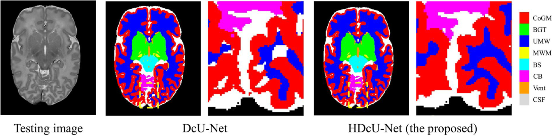
A testing image in NeoBrainS12 and corresponding segmentation results by the DcU-Net without harmonization and with harmonization (the proposed method), with zoomed views.

Table 4.

Results of different methods on NeoBrainS12 challenge data. The highest DC and lowest MSD/HD are indicated in bold. The methods marked with symbol “*” have been evaluated over three images initially available for the web-based challenge. The methods marked with symbol “**” had more image and reference data available than provided by the challenge.

Team Name	UWM			MWM			CoGM			CSF
	DC	MSD	HD	DC	MSD	HD	DC	MSD	HD	DC	MSD	HD
UNC-IDEA-II	0.94	0.09	10.57	0.53	0.60	9.19	0.89	0.10	18.79	0.85	0.16	8.66
INFANT-INSIGHT	0.93	0.11	12.40	0.51	0.73	11.42	0.88	0.14	22.56	0.83	0.19	9.42
LRDE_LTCI	0.93	0.11	20.63	0.06	5.84	20.74	0.87	0.11	26.02	0.83	0.20	10.15
ISI-Neo2**	0.93	0.12	13.81	0.56	0.68	21.23	0.87	0.11	16.11	0.83	0.19	9.67
Anonymous2	0.92	0.14	6.38	–	–	–	0.87	0.13	7.29	0.68	0.61	14.60
UPF_SIMBioSys	0.91	0.17	5.90	0.54	0.62	20.62	0.85	0.15	6.56	0.79	0.29	9.71
FER-UMCU**	0.91	0.17	6.55	0.60	0.59	9.74	0.86	0.13	5.15	0.77	0.33	10.01
ImperialTeam1	0.90	0.18	7.04	–	–	–	0.85	0.17	9.41	0.79	0.32	11.31
DTC	0.89	0.22	6.23	0.47	0.88	12.61	0.84	0.16	5.53	0.76	0.35	9.63
UMCU1**	0.89	0.21	6.95	0.60	0.52	14.84	0.84	0.13	7.70	0.75	0.34	11.53
MCRI	0.88	0.25	8.05	–	–	–	0.84	0.19	8.61	0.73	0.56	10.94
UCL*	0.87	0.26	30.23	0.23	9.41	42.71	0.83	0.18	6.11	0.71	0.54	12.47
Picsl_upenn*	0.85	0.38	14.13	0.33	3.64	30.20	0.80	0.27	27.72	0.61	0.74	15.40
DCU*	0.83	0.40	14.65	–	–	–	–	–	–	–	–	–
UNC-IDEA*	–	–	–	–	–	–	0.86	0.11	4.78	–	–	–
DcU-Net	0.93	0.11	15.32	0.53	0.62	9.29	0.88	0.10	20.46	0.84	0.19	9.21
HDcU-Net (the proposed)	0.94	0.09	10.16	0.54	0.58	9.27	0.89	0.10	18.90	0.85	0.17	8.66
Team Name	UWM			MWM			CoGM			CSF
	DC	MSD	HD	DC	MSD	HD	DC	MSD	HD	DC	MSD	HD
UNC-IDEA-II	0.90	0.14	13.76	0.95	0.26	16.40	0.86	0.24	7.13	0.94	0.30	19.84
INFANT-INSIGHT	0.89	0.15	14.91	0.92	0.51	27.61	0.82	0.32	14.10	0.91	0.56	24.53
LRDE_LTCI	0.87	0.24	12.76	0.94	0.33	14.74	0.85	0.49	13.63	0.91	0.51	16.85
FER-UMCU**	0.86	0.32	10.97	0.93	0.33	5.61	0.88	0.19	3.54	0.93	0.29	4.63
UMCU1**	0.86	0.18	14.70	0.93	0.31	7.47	0.87	0.22	6.48	0.94	0.23	4.35
Anonymous2	0.83	0.24	7.65	–	–	–	–	–	–	0.91	0.62	7.84
UPF_SIMBioSys	0.83	0.44	10.72	0.94	0.28	5.40	0.85	0.15	6.56	0.93	0.29	5.29
ImperialTeam1	0.81	1.38	29.65	0.92	0.43	6.23	0.83	0.56	6.00	0.90	0.62	7.68
DTC	0.85	0.22	9.50	0.92	0.41	6.99	0.78	0.37	4.69	0.88	0.47	6.28
MCRI	–	–	–	0.90	0.57	8.55	0.79	0.69	24.77	0.88	0.70	21.51
ISI-Neo2**	0.81	0.43	22.76	0.93	1.14	61.17	0.85	0.35	42.96	0.91	0.46	23.98
UCL*	0.81	0.32	9.39	0.90	0.53	7.85	0.82	0.80	46.51	0.89	0.56	30.19
Picsl_upenn*	0.86	0.22	17.15	0.91	0.55	26.90	0.74	0.83	22.07	0.80	1.25	21.51
DCU*	–	–	–	–	–	–	–	–	–	–	–	–
UNC-IDEA*	–	–	–	0.92	0.45	5.78	0.83	0.27	3.33	0.92	0.33	4.32
DcU-Net	0.87	0.32	23.94	0.95	0.28	20.28	0.85	0.25	3.64	0.93	0.32	17.38
HDcU-Net (the proposed)	0.89	0.14	14.51	0.95	0.25	16.08	0.86	0.23	7.13	0.94	0.28	19.50

4.5. Results on cross-site and cross-time datasets

The proposed method can also handle cross-site and cross-time datasets. As we know, the tissue contrast for MR image is extremely low at 6-month-old of age due to brain dynamic and rapid changes including myelination [9]. Consequently, it is even challenging for manual segmentation. However, compared with 6-month-old infant images, 24-month-old infant images show a better tissue contrast, and we can easily use existing tools, like FreeSurfer [30], for generating reliable segmentations. For example, Fig. 8(a) is a 24-month-old infant brain MR image (from Baby Connectome Project, BCP) with a good tissue contrast, while Fig. 8(b) is a 6-month-old infant brain MR image (from National Database for Autism Research, NDAR) with a low tissue contrast. The parameters of data acquisition for two datasets are shown in Table 5. Therefore, we considered 24-month-old images from BCP as the source domain and 6-month-old images from NDAR as the target domain, and leveraged the proposed harmonization to transfer labels from 24-month-old subjects into 6-month-old subjects. Specifically, eight 24-month-old images with labels from FreeSurfer were used for training tissue segmentation model; ten 24-month-old images from BCP and ten 6-month-old images from NDAR were used for training CycleGAN model. These 24-month-old infant images were first linearly aligned with one randomly selected 6-month-old infant image, to alleviate the resolution and shape differences. Finally, the models were tested on ten 6-month-old images from NDAR. Note that the ten 6-month-old testing subjects are different from the ten 6-month-old images employed for the CycleGAN training.

Fig. 8.

The tissue contrast comparison for MR images from cross-time datasets. (a) 24-month-old infant image with good tissue contrast from BCP. (b) 6-month-old infant image with extremely low tissue contrast from NDAR.

Table 5.

Parameters of data acquisition for Baby Connectome Project and National Database for Autism Research.

Datasets	Age	Scanner	TR (ms)	TE (ms)	Resolution (mm3)
Source: BCP – 24 months	24-month	Siemens 3T	1,900	4.38	0.8 × 0.8 × 0.8
Target: NDAR – 6 months	6-month	Siemens 3T	2,400	3.16	1.0 × 1.0 × 1.0

Fig. 9 shows the comparisons of results by different methods on a 6-month-old subject. The first two rows show the target image and corresponding segmentation results by the U-Net and the DcU-Net. As the intensity distribution for 6-month-old infant brain MR images is quite different from 24-month-old images, the segmentation result is unacceptable. The third and fourth rows show harmonized images and corresponding segmentation results by the harmonized U-Net and the HDcU-Net. It can be observed that the results are greatly improved.

Fig. 9.

Comparisons of results without/with harmonization on 6-month-old MR image in the target domain. The first and second rows show the target image from NDAR and corresponding segmentation results through the U-Net and the DcU-Net respectively. The third and fourth rows show the harmonized image and corresponding segmentation results by harmonized U-Net and HDcU-Net respectively. The fifth row shows the manual segmentation.

For a quantitative comparison, we evaluated ten 6-month-old images from the target dataset. The average DC and MHD for the results without/with the harmonization are presented in Table 6. It can be seen that the harmonization strategy achieves a higher Dice coefficient and has lower MHD values in terms of WM, GM and CSF, especially with a strong significantly difference compared with other methods as shown in Table 7 ({WM, GM, CSF}/DC: p-value<0.01).

Table 6.

Averaged Dice coefficient (in percentage) and MHD (in mm) for different methods for tissue segmentation of ten 6-month-old MR images in NDAR dataset.

Method	Tissue	U-Net	Harmonized U-Net	DcU-Net	HDcU-Net (the proposed)
DC	WM	56.64±10.76	76.24±3.35	61.58±9.81	80.06±3.34
	GM	71.90±3.05	76.54±2.67	72.00±3.38	79.40±2.63
	CSF	83.57±1.40	79.82±1.91	80.76±2.11	82.73±1.78
MHD (in mm)	WM	6.82±1.56	2.26±0.13	7.50±2.07	2.11±0.26
	GM	2.32±0.60	1.56±0.25	3.00±0.82	1.48±0.13
	CSF	2.50±0.72	2.47±0.45	3.94±0.94	2.05±0.49

Table 7.

The p-value of t-test between the results of any two methods for {WM, GM, CSF}/DC.

Methods	U-Net	Harmonized U-Net	DcU-Net	HDcU-Net (the proposed)
U-Net	-	3.2 × 10−4+/3.2 × 10−6+/2.6 × 10−6+	1.8 × 10−6+/0.561/1.4 × 10−5+	4.8 × 10−6+/5.0 × 10−9+/0.005+
Harmonized U-Net		-	1.1 × 10−4+/6.6 × 10−6+/0.167	4.4 × 10−7+/4.7 × 10−9+/3.0 × 10−8+
DcU-Net			-	1.1 × 10−5+/2.9 × 10−8+/0.003+
HDcU-Net (the proposed)				-

⁺Denotes strong statistical significance (p-value<0.01). The value in each cell represents the p-values for WM/DC, GM/DC and CSF/DC respectively.

5. Discussions and conclusion

In this article, we are not aiming to propose a new segmentation architecture. Instead, we aim to propose a harmonized strategy to improve segmentation performance for infant brain MR images in cross-site datasets scenarios. As a result, the segmentation model employed in the paper can be replaced with any classic architecture for tissue segmentation.

Note that in this paper we assume that there are no labels in the target domain. If the labels in the target domain were available, we could directly train the segmentation model based on the subjects with labels in the target domain and apply to the remaining subjects in the target domain. To test whether our proposed harmonization segmentation from the source domain to the target domain is comparable with direct training/testing in the target domain, we made a comparison of their performances on the same 8 subjects from Section 4.2 in Table 8, in which the DcU-Net model was directly trained in the target domain. It can be seen that direct training in the target domain did achieve a better performance in terms of DC. However, there is no statistical difference in terms of MHD, e.g., WM/MHD: p-value = 0.351, GM/MHD: p-value = 0.322. Although the performance in terms of DC is degraded, it does not mean that our proposed harmonization segmentation is useless since the reliable labels are not always available in the target domain, especially when the manual annotation is difficult, expensive, and time-consuming for the low contrast images, like 6-month-old subjects in Section 4.5. For the same reason, although using the data with real artifacts would be better for validating the performance of the proposed method in Section 4.3, the ground truth of MR images with real artifacts, especially with severe artifacts, are difficult for manual annotation even for experienced neuroradiologist. Furthermore, our generated labels on the to-be-segmented datasets can be further employed for semi-supervised learning [31–34], weakly-supervised learning [35–37] and self-learning [38,39]. Besides, the proposed method is also suitable for the images with different intensity distribution even in the same dataset. For example, in NeoBrainS12, different images are acquired in different gestation corrected ages, which result in different intensity distributions.

Table 8.

Averaged Dice coefficient (in percentage) and MHD (in mm) on 8 neonatal MR images by the models trained in the source domain and the target domain.

Method	DC			MHD (in mm)
	WM	GM	CSF	WM	GM	CSF
HDcU-Net (trained in the source domain)	93.79±0.67	86.95±0.60	87.35±0.96	0.95±0.02	1.08±0.37	1.89±0.26
DcU-Net (trained in target domain)	96.61±0.48	93.20±0.51	94.21±1.35	0.94±0.00	0.94±0.00	0.94±0.00

We also compared with other domain adaption methods. As shown in Fig. 10, SynSeg-Net [17] cannot achieve an accurate segmentation on the same subject in Section 4.2, with Dice coefficient of WM only around 71 %. The poor performance of the SynSeg-Net is mainly due to that the SynSeg-Net is working on 2D slices instead of 3D volume. Although our proposed method can produce encourage segmentation results for neonatal subjects from cross-sites, it still has several limitations: (1) we only considered to harmonize all the target sites to the source site, which could result in the site bias issue; (2) we only validated the method on a small dataset. The reason is that manual annotation for ground truth is time-consuming and expensive, e.g., 6-month-old brain image is pretty difficult for manual segmentation because of the extremely low contrast between gray matter and white matter. That is the reason why we proposed the harmonization segmentation model which was trained on a dataset with manual annotation and can be robustly applied on other datasets without any manual annotation. Accordingly, in our future work, (1) we plan to map image from all sites into a latent space and perform segmentation in the latent space to maximally alleviate the site bias issue [40]; (2) we will increase the number of training/validation images for more robust training and validation. Besides, as discussed in [41] and [42], unpaired training does not have the data fidelity loss term, therefore there is no guarantee of preservation of small abnormality regions during the translation process and direct interpretation of generated images should be taken with caution. Our proposed method introduces the CycleGAN for domain adaptation, which is aiming at improving segmentation results for neonatal brain MR images, instead of improving image quality.

Fig. 10.

Comparison results between SynSeg-Net and the proposed method. Figures from left to right are the original image, the segmentation results by SynSeg-Net and the proposed method, the ground truth with 3D rendering results.

In conclusion, we proposed a novel harmonized neonatal brain MR images segmentation method. Aiming at improving the segmentation performance for cross-site datasets scenarios, we took advantage of CycleGAN which can harmonize images from target domain to source domain, and also alleviate imaging artifacts caused during MR image scanning, such as motion. Finally, the DcU-Net-based segmentation model trained in the source domain can be applied directly on the harmonized images after CycleGAN. The experimental results have demonstrated that the segmentation performance is improved significantly by the proposed method.

References

- [1].Wang L, Gao Y, Shi F, Li G, Gilmore JH, Lin W, Shen D, LINKS: Learning-based multi-source IntegratioN frameworK for Segmentation of infant brain images, NeuroImage 108 (2015) 160–172, 10.1016/j.neuroimage.2014.12.042. [DOI] [PMC free article] [PubMed] [Google Scholar]
- [2].Li G, Wang L, Yap P-T, Wang F, Wu Z, Meng Y, Dong P, Kim J, Shi F, Rekik I, Lin W, Shen D, Computational neuroanatomy of baby brains: a review, NeuroImage 185 (2019) 906–925, 10.1016/j.neuroimage.2018.03.042. [DOI] [PMC free article] [PubMed] [Google Scholar]
- [3].Çiçek Ö, Abdulkadir A, Lienkamp SS, Brox T, Ronneberger O, 3D U-Net: learning dense volumetric segmentation from sparse annotation, International Conference on Medical Image Computing and Computer-Assisted Intervention (2016) 424–432, 10.1007/978-3-319-46723-8_49. [DOI] [Google Scholar]
- [4].Qi K, Yang H, Li C, Liu Z, Wang M, Liu Q, Wang S, X-Net: brain stroke lesion segmentation based on depthwise separable convolution and long-range dependencies, International Conference on Medical Image Computing and Computer-Assisted Intervention (2019) 247–255, 10.1007/978-3-030-32248-9_28. [DOI] [Google Scholar]
- [5].Yang H, Huang W, Qi K, Li C, Liu X, Wang M, Zheng H, Wang S, CLCI-Net: cross-level fusion and context inference networks for lesion segmentation of chronic stroke, International Conference on Medical Image Computing and Computer-Assisted Intervention (2019) 266–274, 10.1007/978-3-030-32248-9_30. [DOI] [Google Scholar]
- [6].Zhou Y, Huang W, Dong P, Xia Y, Wang S, D-UNet: a dimension-fusion U shape network for chronic stroke lesion segmentation, IEEE/ACM Transactions on Computational Biology and Bioinformatics (2019), 10.1109/TCBB.2019.2939522, 1–1. [DOI] [PubMed] [Google Scholar]
- [7].Zhang W, Li R, Deng H, Wang L, Lin W, Ji S, Shen D, Deep convolutional neural networks for multi-modality isointense infant brain image segmentation, NeuroImage 108 (2015) 214–224, 10.1016/j.neuroimage.2014.12.061. [DOI] [PMC free article] [PubMed] [Google Scholar]
- [8].Nie D, Wang L, Gao Y, Shen D, Fully convolutional networks for multi-modality isointense infant brain image segmentation, IEEE 13th International Symposium on Biomedical Imaging (2016) 1342–1345, 10.1109/ISBI.2016.7493515. [DOI] [PMC free article] [PubMed] [Google Scholar]
- [9].Wang L, Nie D, Li G, Puybareau E, Dolz J, Zhang Q, Wang F, Xia J, Wu Z, Chen J, Thung K-H, Bui TD, Shin J, Zeng G, Zheng G, Fonov VS, Doyle A, Xu Y, Moeskops P, Pluim JPW, Desrosiers C, Ayed IB, Sanroma G, Benkarim OM, Casamitjana A, Vilaplana V, Lin W, Li G, Shen D, Benchmark on automatic 6-month-old infant brain segmentation algorithms: the iSeg-2017 challenge, IEEE Trans. Med. Imaging 38 (2019) 2219–2230, 10.1109/TMI.2019.2901712. [DOI] [PMC free article] [PubMed] [Google Scholar]
- [10].Sun Y, Gao K, Wu Z, Lei Z, Wei Y, Ma J, Yang X, Feng X, Zhao L, Phan T, Shin J, Zhong T, Zhang Y, Yu L, Li C, Basnet R, Ahmad M, Swamy M, Ma W, Wang L, Multi-site infant brain segmentation algorithms: the iSeg-2019 challenge, IEEE Trans. Med. Imaging (2021), 10.1109/TMI.2021.3055428, 1–1. [DOI] [PMC free article] [PubMed] [Google Scholar]
- [11].Bousmalis K, Silberman N, Dohan D, Erhan D, Krishnan D, Unsupervised pixel-level domain adaptation with generative adversarial networks, IEEE Conference on Computer Vision and Pattern Recognition (2017) 3722–3731, 10.1109/CVPR.2017.18. [DOI] [Google Scholar]
- [12].Tzeng E, Hoffman J, Saenko K, Darrell T, Adversarial discriminative domain adaptation, IEEE Conference on Computer Vision and Pattern Recognition (2017) 7167–7176, 10.1109/CVPR.2017.316. [DOI] [Google Scholar]
- [13].Sun B, Feng J, Saenko K, Return of frustratingly easy domain adaptation, Thirtieth AAAI Conference on Artificial Intelligence (2016) 2058–2065. [Google Scholar]
- [14].Ganin Y, Ustinova E, Ajakan H, Germain P, Larochelle H, Laviolette F, Marchand M, Lempitsky V, Domain-adversarial training of neural networks, J. Mach. Learn. Res. 17 (2016), 2096–2030. [Google Scholar]
- [15].Tzeng E, Hoffman J, Darrell T, Saenko K, Simultaneous deep transfer across domains and tasks, IEEE International Conference on Computer Vision (2015) 4068–4076, 10.1109/ICCV.2015.463. [DOI] [Google Scholar]
- [16].Sadda P, Onofrey JA, Papademetris X, Deep learning retinal vessel segmentation from a single annotated example: an application of cyclic generative adversarial neural networks, International Workshop on Large-Scale Annotation of Biomedical Data and Expert Label Synthesis (2018) 82–91, 10.1007/978-3-030-01364-6_10. [DOI] [Google Scholar]
- [17].Huo Y, Xu Z, Moon H, Bao S, Assad A, Moyo TK, Savona MR, Abramson RG, Landman BA, SynSeg-Net: synthetic segmentation without target modality ground truth, IEEE Trans. Med. Imaging 38 (2019) 1016–1025, 10.1109/TMI.2018.2876633. [DOI] [PMC free article] [PubMed] [Google Scholar]
- [18].Huo Y, Xu Z, Bao S, Assad A, Abramson RG, Landman BA, Adversarial synthesis learning enables segmentation without target modality ground truth, IEEE 15th International Symposium on Biomedical Imaging (2018) 1217–1220, 10.1109/ISBI.2018.8363790. [DOI] [Google Scholar]
- [19].Khalili N, Turk E, Zreik M, Viergever MA, Benders MJNL, Isgum I, Generative adversarial network for segmentation of motion affected neonatal brain MRI, International Conference on Medical Image Computing and Computer-Assisted Intervention (2019) 320–328, 10.1007/978-3-030-32248-9_36. [DOI] [Google Scholar]
- [20].Dewey BE, Zhao C, Reinhold JC, Carass A, Fitzgerald KC, Sotirchos ES, Saidha S, Oh J, Pham DL, Calabresi PA, van Zijl PCM, Prince JL, DeepHarmony: a deep learning approach to contrast harmonization across scanner changes, Magn. Reson. Imaging 64 (2019) 160–170, 10.1016/j.mri.2019.05.041. [DOI] [PMC free article] [PubMed] [Google Scholar]
- [21].Dong N, Kampffmeyer M, Liang X, Wang Z, Dai W, Xing E, Unsupervised domain adaptation for automatic estimation of cardiothoracic ratio, International Conference on Medical Image Computing and Computer-Assisted Intervention (2018) 544–552, 10.1007/978-3-030-00934-2_61. [DOI] [Google Scholar]
- [22].Wang J, Huang H, Chen C, Ma W, Huang Y, Ding X, Multi-sequence cardiac MR segmentation with adversarial domain adaptation network, International Workshop on Statistical Atlases and Computational Models of the Heart (2019) 254–262, 10.1007/978-3-030-39074-7_27. [DOI] [Google Scholar]
- [23].Kuling G, Curpen B, Martel A, Domain adapted breast tissue segmentation in magnetic resonance imaging, 15th International Workshop on Breast Imaging (2020), 10.1117/12.2564131, pp. 115131B. [DOI] [Google Scholar]
- [24].Zhou B, Augenfeld Z, Chapiro J, Zhou SK, Liu C, Duncan J, Anatomy-guided multimodal registration by learning segmentation without ground truth: application to intraprocedural CBCT/MR liver segmentation and registration, Med. Image Anal. 71 (2021), 102041, 10.1016/j.media.2021.102041. [DOI] [PMC free article] [PubMed] [Google Scholar]
- [25].Sled JG, Zijdenbos AP, Evans AC, A nonparametric method for automatic correction of intensity nonuniformity in MRI data, IEEE Trans. Med. Imaging 17 (1998) 87–97, 10.1109/42.668698. [DOI] [PubMed] [Google Scholar]
- [26].Wang L, Li G, Shi F, Cao X, Lian C, Nie D, Liu M, Zhang H, Li G, Wu Z, Lin W, Shen D, Volume-based analysis of 6-month-old infant brain MRI for autism biomarker identification and early diagnosis, International Conference on Medical Image Computing and Computer-Assisted Intervention (2018) 411–419, 10.1007/978-3-030-00931-1_47. [DOI] [PMC free article] [PubMed] [Google Scholar]
- [27].Zhu J-Y, Park T, Isola P, Efros AA, Unpaired image-to-image translation using cycle-consistent adversarial networks, IEEE International Conference on Computer Vision (2017) 2380–7504, 10.1109/ICCV.2017.244. [DOI] [Google Scholar]
- [28].He K, Zhang X, Ren S, Sun J, Deep residual learning for image recognition, IEEE Conference on Computer Vision and Pattern Recognition (2016) 770–778, 10.1109/CVPR.2016.90. [DOI] [Google Scholar]
- [29].Isgum I, Benders MJ, Avants B, Cardoso MJ, Counsell SJ, Gomez EF, Gui L, Huppi PS, Kersbergen KJ, Makropoulos A, Melbourne A, Moeskops P, Mol CP, Kuklisova-Murgasova M, Rueckert D, Schnabel JA, Srhoj-Egekher V, Wu J, Wang S, de Vries LS, Viergever MA, Evaluation of automatic neonatal brain segmentation algorithms: the NeoBrainS12 challenge, Med. Image Anal. 20 (2015) 135–151, 10.1016/j.media.2014.11.001. [DOI] [PubMed] [Google Scholar]
- [30].Sabuncu MR, Yeo BTT, Van Leemput K, Fischl B, Golland P, A generative model for image segmentation based on label fusion, IEEE Trans. Med. Imaging 29 (2010) 1714–1729, 10.1109/TMI.2010.2050897. [DOI] [PMC free article] [PubMed] [Google Scholar]
- [31].Huo Y, Xu Z, Aboud K, Parvathaneni P, Bao S, Bermudez C, Resnick SM, Cutting LE, Landman BA, Spatially localized atlas network tiles enables 3D whole brain segmentation from limited data, International Conference on Medical Image Computing and Computer-Assisted Intervention (2018) 698–705, 10.1007/978-3-030-00931-1_80. [DOI] [Google Scholar]
- [32].Enguehard J, O’Halloran P, Gholipour A, Semi supervised learning with deep embedded clustering for image classification and segmentation, IEEE Access 7 (2019) 11093–11104, 10.1109/ACCESS.2019.2891970. [DOI] [PMC free article] [PubMed] [Google Scholar]
- [33].Sun Y, Gao K, Niu S, Lin W, Li G, Wang L, Semi-supervised transfer learning for infant cerebellum tissue segmentation, International Workshop on Machine Learning in Medical Imaging (2020) 663–673, 10.1007/978-3-030-59861-7_67. [DOI] [PMC free article] [PubMed] [Google Scholar]
- [34].Zhou Y, He X, Huang L, Liu L, Zhu F, Cui S, Shao L, Collaborative learning of semi-supervised segmentation and classification for medical images, IEEE/CVF Conference on Computer Vision and Pattern Recognition (2019) 2074–2083, 10.1109/CVPR.2019.00218. [DOI] [Google Scholar]
- [35].Wei Y, Liang X, Chen Y, Shen X, Cheng M-M, Zhao Y, Yan S, STC: a simple to complex framework for weakly-supervised semantic segmentation, IEEE Trans. Pattern Anal. Mach. Intell. 39 (2015) 2314–2320, 10.1109/TPAMI.2016.2636150. [DOI] [PubMed] [Google Scholar]
- [36].Kervadec H, Dolz J, Tang M, Granger E, Boykov Y, Ben Ayed I, Constrained-CNN losses for weakly supervised segmentation, Med. Image Anal. 54 (2019) 88–99, 10.1016/j.media.2019.02.009. [DOI] [PubMed] [Google Scholar]
- [37].Shimoda W, Yanai K, Self-supervised difference detection for weakly-supervised semantic segmentation, International Conference on Computer Vision (2019) 5207–5216, 10.1109/ICCV.2019.00531. [DOI] [Google Scholar]
- [38].Bai W, Chen C, Tarroni G, Duan J, Guitton F, Petersen S, Guo Y, Matthews P, Rueckert D, Self-supervised learning for cardiac MR image segmentation by anatomical position prediction, International Conference on Medical Image Computing and Computer-Assisted Intervention (2019) 541–549, 10.1007/978-3-030-32245-8_60. [DOI] [Google Scholar]
- [39].Sun Y, Gao K, Ying S, Lin W, Li G, Niu S, Liu M, Wang L, Self-supervised transfer learning for infant cerebellum segmentation with multi-domain MRIs, International Society for Magnetic Resonance in Medicine, 2021. [Google Scholar]
- [40].Choi Y, Choi M, Kim M, Ha J-W, Kim S, Choo J, StarGAN: unified generative adversarial networks for multi-domain image-to-Image translation, IEEE Conference on Computer Vision and Pattern Recognition (2018) 8789–8797, 10.1109/CVPR.2018.00916. [DOI] [Google Scholar]
- [41].Yi X, Walia E, Babyn P, Generative adversarial network in medical imaging: a review, Med. Image Anal. 58 (2019), 101552, 10.1016/j.media.2019.101552. [DOI] [PubMed] [Google Scholar]
- [42].Cohen JP, Luck M, Honari S, Distribution matching losses can hallucinate features in medical image translation, International Conference on Medical Image Computing and Computer-Assisted Intervention (2018) 529–536, 10.1007/978-3-030-00928-1_60. [DOI] [Google Scholar]
Associated Data
This section collects any data citations, data availability statements, or supplementary materials included in this article.