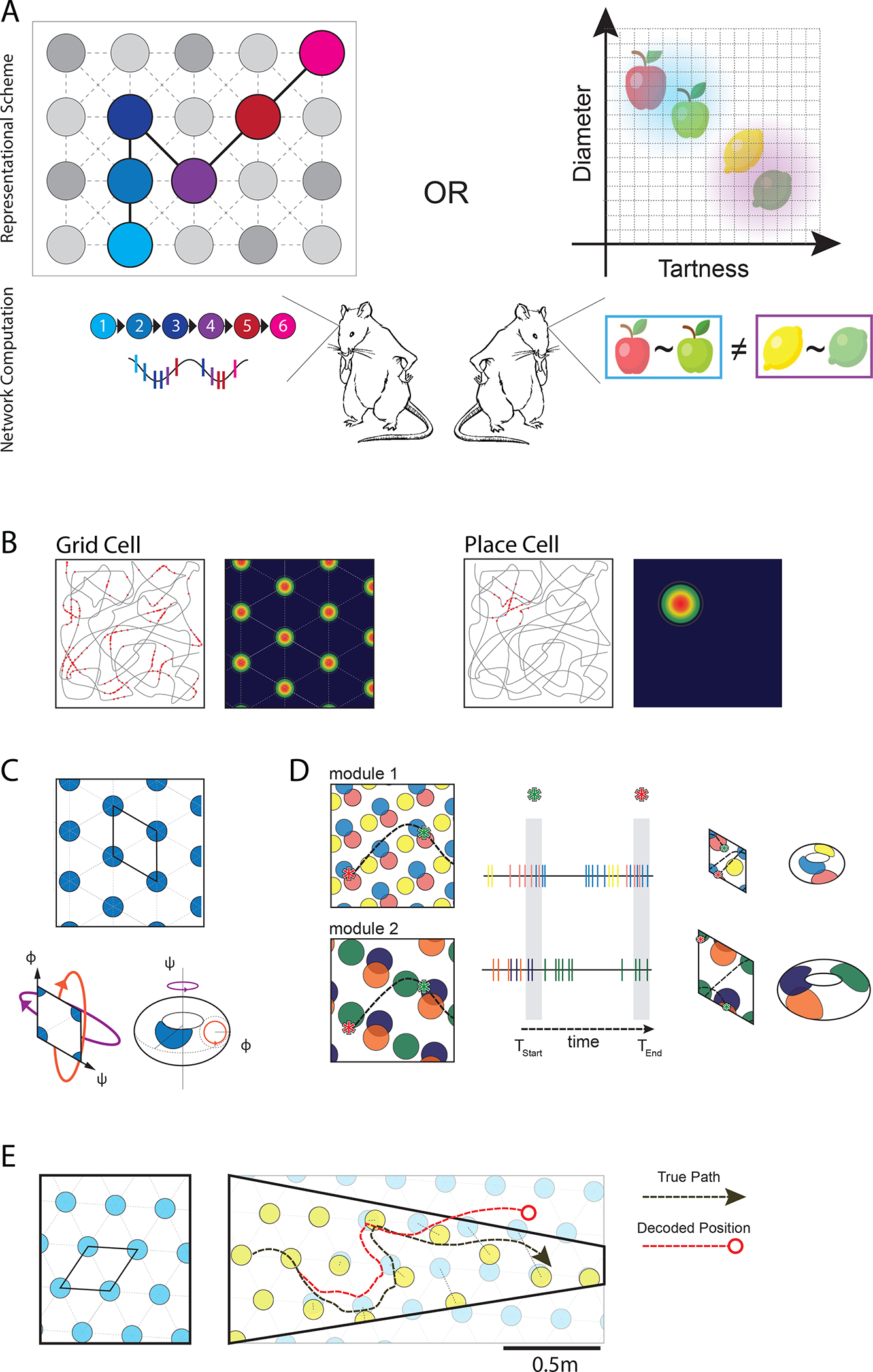
Figure 1. Representations argued to be supported by grid cells.

A) Comparison of conceptual models that may be supported by grid cells. The ‘Representational Scheme’ illustrates how the entorhinal-hippocampal network represents relationships (top), and the ‘Network Computation’ illustrates the nature of the information supplied to readers of the entorhinal-hippocampal network (bottom). Left: Topology based in temporal order. Structure across nodes is rooted in the order of events in experience; relationships reflect temporal adjacency. This structure formulates sequences that can link disparate items, which may be manifest in the fine timing of spikes within each theta cycle (see Fig. 2). Right: Feature space defined by axes that quantify featural attributes of items. Relationships between items are defined by the qualities measured within the feature space, which can be used to derive categories (e.g. types of apples or citrus fruits; see Box 2).

B) Firing patterns of an archetypical grid cell in MEC (left) and place cell in hippocampus (right) in a square open arena. Grey line depicts the trajectory of the animal; red dots are spikes. The spatially averaged firing rates of the cells are shown with warmer colors indicating higher firing rates.

C) Grid cell fields are organized in a rhombus-shaped tile that spans the environment. Relative position within the tile is given by coordinates (phi, psi) defined by the rhombus axes. In one proposed implementation of connectivity within the tile, connecting the rhombus edges forms a twisted torus^19,20,50,51, creating a continuous surface capable of generating periodic fields.

D) Grid cells with similar field spacing and orientation are organized in modules. Spatial offset between grid cells indexes relative position within a module tile. Combining activity across modules disambiguates individual positions in the environment (trajectory: dotted line). Spike rasters demonstrate the activity of each module over time as the trajectory progresses. The population rate code across modules creates a unique identifier for each position in space (green and red stars).

E) Inaccurate decoded positions resulting from distortion in grid field spacing (adapted from ⁶⁴).