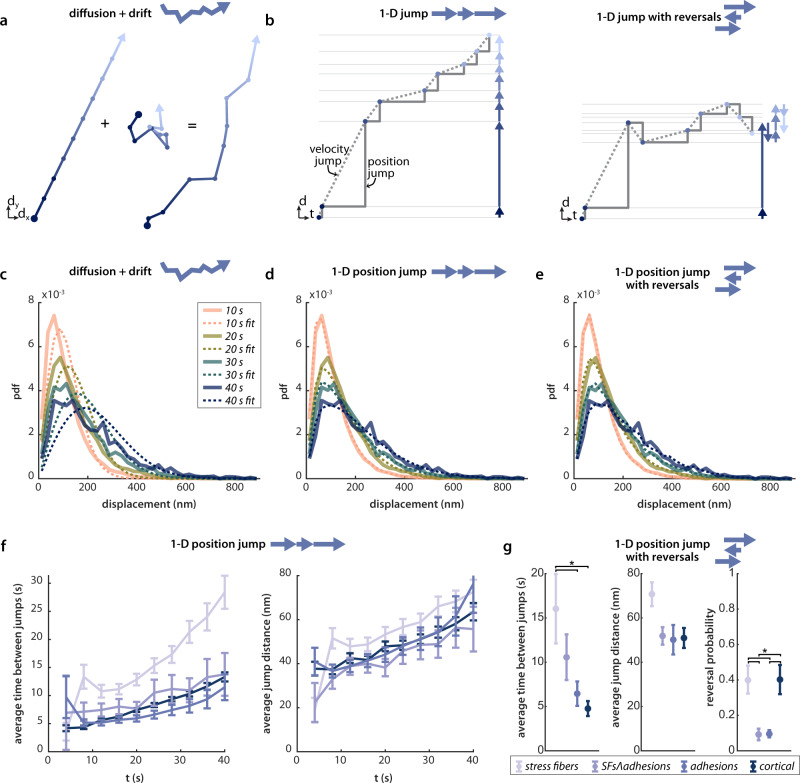
Fig. 4. F-actin velocity distributions in HFFs are well-fit by a jump process model with exponentially distributed waiting times and jump distances.

a Schematic of the diffusion with drift model. Persistent drift (left) is coupled with diffusion (center), leading to the motion shown on the right. b Schematic of the jump model, both with (right) and without (left) direction reversals. The one-dimensional motion is shown both in two-dimensional distance-time space and in one-dimensional space (arrows). The solid lines represent the motion of a position jump model, while the dashed lines represent the analogous velocity jump model. c–e The best fits to the stress fiber population data by each of the models in a and b: diffusion with drift (c), 1-D position jump (d), and 1-D position jump with reversals (e). The fits are shown for four timescales and are for representative data from one experiment (n = 9 cells). f The best fit parameters for the 1-D jump process, for all timescales measured, averaged over four experiments. Error bars show 95% confidence intervals on the fit parameters, propagated across the four datasets (see Methods, Model Fitting for details). g The best fit parameters for the 1-D jump process with reversals, fit to all timescales (2–40 s), averaged over four experiments, n = 32 total cells. Error bars show standard error of the mean of the fit parameters from four independent datasets. Groups were compared with one-way ANOVA and asterisks denote comparisons with p-values < 0.05. P-values for comparisons between all groups are tabulated in Supplementary Table 3. Source data for c–g are provided in the Source Data file.