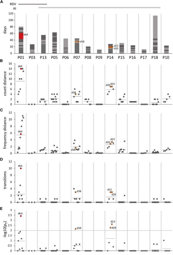
Figure 1.

Cross-comparison of NV diversity in longitudinal patient samples

(A) Overview of sequenced samples with each sample sequenced once, and sample collection time points, relative to the collection date of the first investigated sample. Consecutive longitudinal samples are shown as stacked columns marked in alternating shades of gray, with the height of each segment denoting the time span between sampling dates. Samples exhibiting NV transition counts significantly above the mean expectation value (see below) are shown in orange or red for significance levels of 0.01 or 0.001, respectively, and are additionally labeled with the corresponding sample collection time point.

(B–E) Summary analysis of patient samples. Individual samples are denoted by filled circles, and mean values for each patient are shown as short horizontal lines. (B) and (C) show the aggregated NV distance relative to the first investigated sample, as measured by either the relative number of SNVs with an estimated frequency of at least 1% (B) or the sum of frequency alterations across all SNVs (C). (D) shows the total number of transitions (i.e., events in which SNVs transition from a non-significant or minor to a major state, or vice versa) between consecutive longitudinal samples. (E) shows p values for the hypothesis that the number of transitions observed in a given sample is greater than that expected from the estimated average transition frequency across all samples (pT; see STAR Methods for calculation details). The 0.05 significance cutoff is shown as a horizontal line. Circles filled in blue, orange, or red across all panels denote samples for which this value reaches significance levels of 0.05, 0.01, or 0.001, respectively.