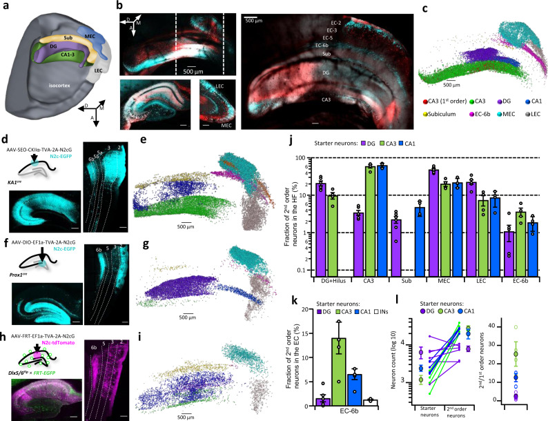
Fig. 2. EC-6b neurons project to all hippocampal sub-regions with a topographic organization.
a 3D schematic overview of the different components comprising the hippocampal formation. A, D, M indicate Anterior, Dorsal, and Medial, respectively. b Intact, cleared cortico-hippocampal preparation following retAAV-assisted labeling from CA3 neurons, as shown in Fig. 1e (red—tdTomato, Cyan—N2c-EGFP; top left), alongside projections of the XY plane along the traced lines (left, bottom) and an annotated image of the preparation in the Z plane (right). c Visual representation of the distribution of N2c-EGFP labeled neurons in the EC and HC, following retrograde labeling from the CA3. d, CA1-specific retrograde labeling scheme (top left) and representative confocal images of the HC (bottom left) and EC (right). e Same as c but for retrograde labeling from the CA1. f DGC-specific retrograde labeling scheme (top left) and representative confocal images of the HC (bottom left) and EC (right). g Same as c but for retrograde labeling from the DG. h CA1 IN-specific retrograde labeling scheme (top left) and representative confocal images of the HC (bottom left) and EC (right). i, Same as c but for retrograde labeling from hippocampal interneurons. j Labeling distribution across cortico-hippocampal sub-regions following retrograde labeling from the CA3, CA1, and DG. Fraction in each region was calculated separately for each condition of the total number of 2nd order neurons. k Fraction of entorhinal SPNs out of the total number of projection neurons in the EC, following retrograde labeling from the CA3, CA1, DG, and hippocampal interneurons. l Numbers of 2nd and 1st order neurons for each starter population (left) along with a summary plot of the calculated ratios of 2nd to 1st order neurons (right). For all calculations, the number of CA3 and mossy cells was multiplied by 2 to account for the number of commissural projection neurons. For DG, n = 6, for all other conditions, n = 4 mice. Unless indicated otherwise, scale bars represent 200 µm. Image in a was acquired using the Allen Institute’s Brain Explorer 2™. Data in j-l is shown as mean and SEM with individual data points shown for each experiment.

