Figure 2.

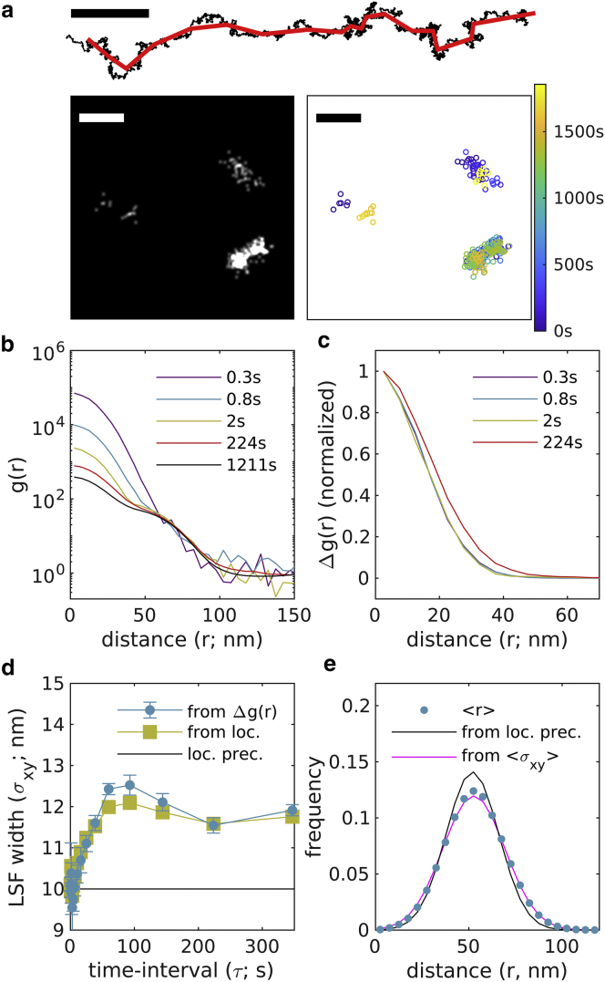
Validation of approach through simulation with drift and drift correction. (a) The simulation from Fig. 1 with applied drift (black) and drift correction (red) as shown in the trajectory above. Reconstructed image (left; 1 nm pixels, 3 nm Gaussian blur) and scatterplot of localizations with color representing the observation time (right) for a small subset of the simulated plane. Scale bar, 100 nm. (b) Autocorrelations as a function of displacement $g(r,\tau )$, tabulated from simulations for time interval windows centered at the values shown. (c) $\text{Δ}g\left(r,\tau \right)=g\left(r,\tau \right)-g\left(r,{\tau }_{\max }=1211s\right)$ for the examples shown in (b). (d) $\Delta g(r,\tau )$ are fit to $\text{Δ}g\left(r,\tau \right)\propto \exp \left\{-r^2/4{\sigma }_{xy}^2\right\}$ to extract the width of the effective LSF in each lateral dimension. In this case, the LSF width varies with time interval, closely following the LSF width measured by grouping localizations with molecules (from loc.). Error bars represent estimates of the standard error obtained through bootstrapping. (e) The distribution of displacements between different molecules on the same ruler are well described by a model incorporating the average LSF width ($⟨{\sigma }_{xy}⟩=11.8\text{nm}$) and the known separation distance (50 nm). To see this figure in color, go online.