. 2022 Jul 28;11:e71032. doi: 10.7554/eLife.71032

Figure 3. Multipole analysis of the matrix deformation rate.

(a) Snapshots of a cell with: matrix rate of deformation, green arrows, the main dipole axis, blue, the axis of the cell motion, red. (b) Schematic representation of dipoles (D) and quadrupoles (Q) of the 1D matrix displacement (rate) distributions. The distribution on top has non-zero dipole but vanishing quadrupole, and that on the bottom has vanishing dipole and non-zero quadrupole. (c) Time series of the main dipole, blue, and quadrupole, magenta – projected on the cell axis – for a migrating cell (squares) and a non-migrating cell (circles), sampling approximately 1/10 of the duration of the entire experiment. (d–e) Cell trajectory in the dipole/quadrupole phase space for a migrating cell (d) and a non-migrating cell (e). The migrating cell follows a cycle with a finite area and the non-migrating cell does not. The error bars are obtained following the procedure described in Appendix 2. The individual cycles for different radii are shown in light gray. (f) Snapshots of a cell which in the course of the same experiment displays a transition from migrating to non-migrating behavior (LifeAct in red and fibronectin in yellow), scale bar 10 µm. (g) Cell positions in the x-y plane (blue and orange curves) showing a transition from migrating to non-migrating phase. (h) Trajectories in the dipole/quadrupole phase space for three different time intervals showing cycles with finite area in the migrating phase and with vanishing area in the non-migrating phase (see also Video 8).

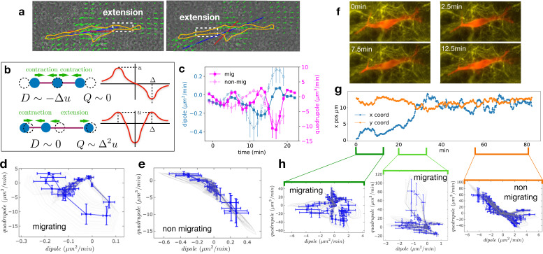
Figure 3—source data 1. Dipole and quadrupole moments.
(i) Raw data for the dipole and quadrupole moments in panel Figure 3d. (ii) Raw data for the dipole and quadrupole moments in panel Figure 3e. (iii) Raw data for the angular distribution.

Figure 3.

Figure 3—figure supplement 1. Method to compute the multipolar terms.

Figure 3—figure supplement 1.

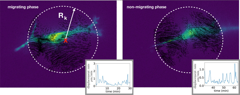
The same cell of Figure 3f in the course of the same experiment shows a transition between migrating phase and non-migrating phase, Figure 3g. Left: Experimental image showing a cell in light blue, and the vector field restricted to a circular region used to compute the multipoles. The center (red cross) is obtained starting from the cell center position and searching for the coordinates (X*, Y*) that minimize the monopole term. We consider regions enclosed by different radii Rk, with k=1, 2,... and compute the multipoles in each of these regions. We then compute the average values of the multipolar terms and obtain error bars as the standard deviations over all these regions. Insets: characteristic scale of matrix displacement rate, computed as the average of the absolute value of the rate of deformation field within the circular region. This quantity is slightly smaller during the non-migrating phase than during the migrating phase but the two values are comparable. Right: The cell does not move because the vector field has changed compared to the migrating phase, showing now mainly a dipolar field.
Figure 3—figure supplement 2. Quantification of cell and dipole orientation.

Figure 3—figure supplement 2.

Histograms of the angle difference δθ between the main dipole axis and the direction of motion (blue and red axes, respectively, in the top-left panel). The full histogram (yellow) is a merge of data from three examples corresponding to Figure 3d, Figure 3h, and the leftmost migrating cell of Figure 3—figure supplement 3 (individual histograms are overlaid in different colors).
Figure 3—figure supplement 3. Quantification of cell motion.

Figure 3—figure supplement 3.

(a) Examples of cell trajectories represented in the dipole/quadrupole phase space. Comparison between cycle curves obtained in different experiments for different migrating (top panels) and non-migrating (bottom panels) cells. We observe a variability in the traction forces for both migrating and non-migrating cells, but we exclude that non-migration is due to lack of traction (compare leftmost top and bottom panels). (b) Average of the matrix displacement rate (same as the inset of Figure 3—figure supplement 1 averaged over time) for the six cells shown in (a). Statistical significance of the differences between the conditions was assessed by a t-test (p=0.2766). (c) Quantification of the area enclosed by the cycles in the dipole/quadrupole space The left panel shows the absolute area in physical units, and the right panel shows the normalized area: the fraction of the area of the rectangle fitting the trajectory of the cycle (see Appendix 2). Statistical significances of the differences between the conditions were assessed by a Kruskal-Wallis test (left panel – p=0.0177) and a t-test (right panel – p=0.0431).