Irregular Shaped Small Nodule Detection Using a Robust Scan Statistic

Abstract

The spatial scan statistics based on the Poisson and binomial models are the most common methods to detect spatial clusters in disease surveillance. These models rely on Monte-Carlo simulation which are time consuming. Moreover, frequently, datasets present over-dispersion which cannot be handled by them. Thus, we have the following goals. First, we propose irregularly shaped spatial scan for the Bell, Poisson, and binomial. The Bell distribution has just one parameter but it is capable of handling over-dispersed datasets. Second, we apply these scan statistics to big maps. A fast version, without Monte-Carlo simulation, for the proposed Poisson and binomial scans is introduced. Intensive simulation studies are carried out to assess the quality of the proposals. In addition, we show the time improvement of the fast scan versions over their traditional ones. Finally, we end the paper with an application on the detection of irregular shape small nodules in a medical image.

Supplementary Information

The online version contains supplementary material available at 10.1007/s12561-022-09353-7.

Introduction

Are points randomly distributed in space or time? This is a common question in almost any field of sciences, for example in astronomy [1, 2], image analysis [3, 4], data mining [5], criminology [6, 7], ecology [8, 9], geography [10, 11], pattern recognition [12], biology [13], forestry [14, 15], epidemiology [16, 17], etc. The answer to this question depends on the position and the number of individuals with some characteristics concerning each other. The final goal is to verify whether “spatial clustering has happened”.

The spatial scan statistic presented by Kulldorff and Nagarwalla [18], is a tool that became popular for the detection and inference of spatial clusters, especially in epidemiology. The detection of disease outbreaks at the earliest possible time is essential for public health centers to develop appropriate public policies. Therefore, the spatial scan statistic is one of the most used statistics to help epidemiologists detect and evaluate spatial clusters in disease surveillance. In summary, this method scans a map with circular windows to determine the most likely zone to be a spatial cluster. Then, using Monte-Carlo simulation determine the significance of this zone.

With the new challenges presented by real data, many extensions over the traditional circular scan statistic [19] was proposed to accommodate large spatial data [4], zero-inflation [20], and over-dispersion and zero-inflation simultaneously [21, 22]. Another common challenge is the detection of the irregularly-shaped cluster. Many works have also been done in this direction [e.g., 23, 24, 25, 26, and others]. Assunção et al. [23] detect irregularly shaped clusters using the minimum spanning tree (MST) from graph theory. The construction of the MST can drastically reduce the number of candidate clusters making the method scalable for larger datasets. However, the method presents an overestimation of the cluster size (the so-called octopus effect). To control the overestimation effect, Costa et al. [24] proposed three spatial scan statistics to find irregularly shaped clusters. These three proposals were constructed upon an early stopping rule, a double connection requirement, and maximum linkage criteria. Another solution was proposed by Zhou et al. [25]. Their method is detailed in Subsect. 2.3.2. For an up-to-date review of scan statistics, we refer to Abolhassani and Prates [27] which includes irregularly shaped scan statistics and many other subjects in this area.

To the best of our knowledge, in epidemiology, it is common for researchers to scan small maps, with less than 1000 counties. This is done in practice because of the large number of candidate circular windows in the scan process and the need for Monte-Carlo hypothesis testing that makes its use of big data inappropriate. In this paper, we have considered a medical image as the study map. The medical image can be considered as a large map. Each pixel of the image can be thought of as a county of a map. The darkness of a pixel corresponds to the number of cases in that pixel. To detect spatial clusters on a medical image (i.e., a big map), we present an irregularly-shaped version of the Poisson, binomial, and Bell scan statistics. Moreover, a fast algorithm to handle big data problems is introduced for the Poisson and binomial scans.

We show by extensive simulation that the irregular Bell is a robust scan alternative to model miss-specification in comparison with the binomial and Poisson models and that the fast scan alternatives can provide about $50\%$ speedup in the computational time in comparison with its traditional Monte-Carlo implementation. Despite the robustness of the irregular Bell scan, we were unable to provide a fast version of its algorithm. When working with event data, Castellares et al. [28] showed that the likelihood calculation time can be drastically reduced. However, this is not related to the goal of the current study.

The rest of this paper is as follows: Sect. 2 provides a broad review of the scan statistics, including in Sect. 2.4 the recent Bell scan statistic that has only one parameter and is suitable for over-dispersed data. An algorithm to detect irregularly-shaped clusters for the Bell distribution with traditional and fast algorithms for binomial and Poisson distributions is presented in Sect. 3. Section 4 presents an intensive simulation study. An application for real data is done in Sect. 5. Finally, we conclude in Sect. 6.

A Review on Scan Statistic

Circular Scan Statistic

Kulldorff [19] proposed a Likelihood Ratio Test (LRT) to detect spatial clusters. To do so, consider an inhomogeneous Poisson point process over k regions or locations in a study area. Let $X_i$ be the number of cases in region i with corresponding at-risk population $n_i$ under unit-specific relative risk ${\zeta }_i$ such that $X_i\sim \text{Poisson}(n_i{\zeta }_i)$. Furthermore, let Z be a subset of indices $1,2,.\dots ,k$, describing a given zone, which represents a candidate cluster. Define $\mathcal{Z}$ as a collection of all candidate clusters. Kulldorff [19] formulated a scan statistic that compares the total number of case-counts in zone Z, $X_Z={\sum }_{i\in Z}{X}_i$, against the total number of case-counts in $\overline{Z}$ (i.e. the zone defined by the areas of the map not in Z), $X_{\overline{Z}}={\sum }_{i\in \overline{Z}}{X}_i$, controlled by the corresponding population counts, that are, $n_Z={\sum }_{i\in Z}{n}_i$ and $n_{\overline{Z}}={\sum }_{i\in \overline{Z}}{n}_i$ within and without zone Z, respectively. Let $n=n_Z+n_{\overline{Z}}$ and $X=X_Z+X_{\overline{Z}}$, and assume that ${\zeta }_i={\zeta }_Z$ for every region $i\in Z$ and that ${\zeta }_i={\zeta }_{\overline{Z}}$ for every region $i\in \overline{Z}$. The hypothesis of interest is given by

$$\begin{array}{c}\hfill H_0:\forall Z\in \mathcal{Z},{\zeta }_Z={\zeta }_{\overline{Z}}={\zeta }_0,\text{vs}{H}_1:\exists Z\in \mathcal{Z}\text{such that}{\zeta }_Z>{\zeta }_{\overline{Z}},\end{array}$$ 1

where $H_0$ implies that there is a constant risk, while $H_1$ implies that there is at least one cluster defined by a zone $Z\in \mathcal{Z}$ such that ${\zeta }_Z>{\zeta }_{\overline{Z}}$. Thus, for every candidate cluster Z, the likelihood function $L(Z)=L(Z,{\zeta }_Z,{\zeta }_{\overline{Z}})$ is given by

$$\begin{array}{c}\hfill L(Z)=\prod _{i\in Z}{\displaystyle \frac{e^{-n_i{\zeta }_Z}{(n_i{\zeta }_Z)}^{x_i}}{(x_i)!}}\prod _{j\notin Z}{\displaystyle \frac{e^{-n_j{\zeta }_{\overline{Z}}}{(n_j{\zeta }_{\overline{Z}})}^{x_j}}{(x_j)!}}.\end{array}$$

Additionally, to present how to find the most likely cluster (MLC), Kulldorff [19] developed a LRT defined by:

$$\begin{array}{c}\hfill \lambda (Z)={\displaystyle \frac{{sup}_{{\zeta }_Z>{\zeta }_{\overline{Z}}}L(Z,{\zeta }_Z,{\zeta }_{\overline{Z}})}{{sup}_{{\zeta }_Z={\zeta }_{\overline{Z}}={\zeta }_0}L(Z,{\zeta }_0)}}I({\zeta }_Z>{\zeta }_{\overline{Z}})\end{array}$$ 2

with $\lambda (Z)=1$, if ${\zeta }_Z<{\zeta }_{\overline{Z}}$ that allows to decide whether or not the MLC is statistically significant, meaning whether the area(s) included in the most likely cluster really incorporate(s) an abnormally high number of cases.

The clustering method introduced by Kulldorff [19] is called scan statistic and has some limitations. First, it cannot detect non-circular clusters. Second, the distribution of the test statistic $\lambda$ is unknown. To solve the first limitation, Kulldorff et al. [29] proposed an elliptic spatial scan statistic, but this method does not detect irregularly shaped clusters well. To find irregularly-shaped clusters, the Minimum Spanning Tree (MST) was first introduced [23] and later the Adaptive MST (AMST) method [25]. They not only enabled researchers to find irregularly shaped clusters but also decreased the scanning time of the map in two ways: (1) by decreasing the cardinality of the candidate class, and (2) by applying Linear Time Subset Scan (LTSS) property [30]. More details about these methods are discussed in Sect. 2.3.

The second limitation of the scan statistic was solved by Soltani and Aboukhamseen [31, 32]. They found the exact distribution for $\lambda$ (Sect. 2.2) which allowed us to modify the Poisson and binomial scan introduced by Zhou et al. [25] to a faster alternative. Hence, these modified versions are more adequate to big maps.

Spatial Clustering Without Monte-Carlo

The advantage of Soltani and Aboukhamseen [32] and Aboukhamseen et al. [31] methods were the elimination of Monte-Carlo in the scan statistic procedure. Consider the hypothesis testing (1), and suppose that $G=Z_1\bigcup Z_2\bigcup \cdots \bigcup Z_k$ is the studying region, also $X_{+,Z}$ and $n_{+}(G)$ are the number of points (cases) in Z and G, respectively. Let $A_Z$ be the event that an individual is in a zone Z and $B_{+}$ stands for the event that an individual in G is a case that has characteristic $+$ (for example an infected person). Consider $P_{+|Z}=P(B_{+}|A_Z)$ and let $\mu$ be a counting measure on $(G,\mathcal{F})$ such that $\mu (Z)$ is the number of people in Z and $\mathcal{F}$ is a sigma-field on G containing $Z_1,\cdots ,Z_k$. Both $\mu (Z_i),i=1,\cdots ,k$ and $\mu (G)$ are known. The probability of $A_Z$ is defined as $\nu (Z)=\frac{\mu (Z)}{\mu (G)}$. According to the above notations, Soltani and Aboukhamseen [32] proved that (1) is equivalent to

$$\begin{array}{c}\hfill H_0:P_{Z|+}=\nu (Z)\text{vs}{H}_1:P_{Z|+}>\nu (Z).\end{array}$$ 3

In addition, they found the exact and asymptotic distribution of points in zone Z under null hypothesis $H_0$, as follows:

$$\begin{array}{cc}\hfill X_{+,Z}& \sim Bin(n_{+}(G),\nu (Z)),\hfill \\ \hfill X_{+,Z}& ⟹N(n_{+}(G)\nu (Z),n_{+}(G)\nu (Z)[1-\nu (Z)]),\hfill \end{array}$$

where ($⟹$) denotes convergence in distribution.

According to the above facts, zone Z is a cluster in level $\alpha$ if

$$\begin{array}{c}\hfill z=\frac{\frac{X_{+,Z}}{n_{+}(G)}-\nu (Z)}{\sqrt{\frac{\nu (Z)[1-\nu (Z)]}{n_{+}(G)}}}>z_{\alpha }.\end{array}$$ 4

In this method of cluster detection, one does not need Monte-Carlo hypothesis testing, hence it is quicker than the method of Kulldorff and Nagarwalla [18].

Aboukhamseen et al. [31] developed a spatial scan statistic for a situation in which $n_{+}(G)$ is a random variable from a Poisson distribution with unknown parameter $\lambda (G)$. Also they consider $X_{+,Z}|n_{+}(G)\sim Bin(n_{+}(G),\nu (Z))$. Since $n_{+}(G)$ has Poisson distribution with parameter $\lambda (G)$ and using the marginal distribution of $X_{+,Z}$, they gave a confidence interval for $\nu (Z)$. Based on the value of $\nu (Z)$, one can decide that if the null hypothesis in (3) will be rejected or not. The large discrepancy between the lower limit of the confidence interval and computed statistic $\nu (Z)$ means smaller p-value and hence greater significance of z.

Aboukhamseen et al. [31] proposed

$$\begin{array}{c}\hfill \pm 0.25z_{\alpha /2}+\sqrt{z_{\alpha /2}^2+4n_{+}(G)}\end{array}$$

as a confidence interval for $\lambda (G)$. However, we notice that this formula is not correct and suggest the use of

$$\begin{array}{c}\hfill n_{+}(G)+\frac{1}{2}{z}_{\alpha /2}^2(1\pm \sqrt{1+\frac{4n_{+}(G)}{z_{\alpha /2}^2}})\end{array}$$

to find correct confidence interval for $\lambda (G)$. In this work we use the latter confidence interval.

Irregular-Shape Clusters

Minimum Spanning Tree

As mentioned before, in the scan statistic method [18], the class of candidates (i.e., circular zones) is too big and it is necessary to compute the likelihood ratio too many times. Further, the scan statistic is capable of detecting only circular clusters. Hence, Assunção et al. [23] solved these two undesired problems by using an MST. In their work, they proposed the MST technique to detect irregularly-shaped clusters. The method is as follows:

Consider a map and mark the center of each county by its centroid. Connect any two counties if they are neighbors. Construct an in-directed graph corresponding to the map. Give a weight W(i, j) to each the edge ($v_i,v_j$), where W(i, j) is computed by the Kullback–Liebler (KL) divergence. Weights reflect dissimilarity of density corresponding to counts of cases between two counties. High W(i, j) means high dissimilarity between the density of county i and j.

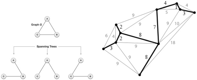
A spanning tree $\tau$ of a graph G is a sub-graph of G which is a tree and contains all nodes of G (Fig. 1 left). The MST is a spanning tree which has the minimum weight. Figure 1 right, shows the representation of an MST. Prim [33] proposed one of the simplest algorithms to build an MST and this method was used by Assunção et al. [23].

Fig. 1.

Left: A Graph and its spanning trees. Right: A graph with weights on edges is in gray color. Black lines show MST

After building the MST, Assunção et al. [23] reduced the class of the candidates from many circular zones to n candidates (n is the number of nodes) by removing one edge at a time from the original MST. In other words, by removing one edge from the MST, two sub-graphs appear. Assunção et al. [23] considered the smallest one as a candidate. Then they return the eliminated edge to its place and remove another edge. Again the smallest sub-graph is considered as the second candidate. This procedure continues until getting the n-th candidate. After obtaining the class of all candidates (with the cardinality of n), they compute $\lambda$ for each element of this class to determine the MLC. In the next step, Monte-Carlo hypothesis testing is used to decide whether the MLC is significant as a cluster or not.

Although the MST method improved the scan statistic in two aspects (i.e., allows flexible shape for the candidate cluster and reduces the class of candidates from a large number of circles to n candidates), it has some deficiencies. First, it just detects one cluster on the map. Second, it tends to detect clusters that are bigger than their actual size. Third, it still requires Monte-Carlo hypothesis testing. To solve the first problem, Zhou et al. [25] introduce the AMST method that is discussed in the following subsection.

Adaptive Minimum Spanning Tree

As mentioned, the MST method detected only one cluster on the map. Although researchers can remove some heavy edges to find two or more clusters, determining the number of elimination is not trivial and is a drawback. To overcome this problem, Zhou et al. [25] proposed the AMST method. In this method, one does not need to have prior knowledge about parameters such as the number of clusters and the initial cluster center.

For the AMST method, the concept of validity index is important and it is defined as:

$${\text{val}}_{\text{index}}={\text{Intra}}_{\text{dist}}/{\text{Inter}}_{\text{dist}},$$ 5

such that ${\text{Intra}}_{\text{dist}}$ measures compactness of sub-partitions of a graph while ${\text{Inter}}_{\text{dist}}$ measures isolation of them, i.e., separation between the sub-partitions.

The Intra cluster distance and Inter cluster distance are defined as follows:

$$\begin{array}{c}\hfill {\text{Intra}}_{\text{dist}}=\sum _{i=1}^K\sum _{j\in C}^{}{|{\lambda }_{C^{\mathit{ij}}}-{\lambda }_{C^i}|}^2/K.\end{array}$$

This is the average of the sum square of the difference of all the incidence rates within a sub-partition, from the rate of that sub-partition. In addition,

$$\begin{array}{c}\hfill {\text{Inter}}_{\text{dist}}=\underset{i,j}{max}{|{\lambda }_{C^i}-{\lambda }_{C^j}|}^2.\end{array}$$

This is the maximum diversification of the point rates of any two sub-partitions with rates ${\lambda }_{C^i}$ and ${\lambda }_{C^j}$. Note that ${\lambda }_{C^i}$ is the expected point rate of sub-partition $C^i$ and ${\lambda }_{C^{\mathit{ij}}}$ is the point rate of county j in candidate sub-partition $C^i$. We call $|{\lambda }_{C^i}-{\lambda }_{C^j}|$ as the distance between sub-partitions i and j. K is the total number of sub-partitions after removing some edges in the minimum spanning tree. One can estimate ${\lambda }_{C^{\mathit{ij}}}$ and ${\lambda }_{C^i}$ by using a maximum likelihood approach. By minimizing ${\text{val}}_{\text{index}}$, the best partition of the MST can be obtained. Then Zhou et al. [25] applied linear time subset scan property (LTSS) [30], on the best partition of the MST to find clusters.

The steps of the algorithm based on the AMST can be found in Zhou et al. [25]. Other proposals for validity indexes are presented in the Supplementary Material Section SM-1 and results were found to be similar to the former one.

The Bell Scan Statistic

Two common classical models to detect spatial clusters are the Poisson and binomial models. Although the Poisson distribution has just one parameter, it has a restriction of having the variance equal to the mean. Hence, this model is not suitable for over-dispersed data sets. In the case of the binomial model, it has two parameters and the index of dispersion (the ratio of variance to the expected value) is less than 1. Considering these facts, the Poisson and binomial distributions may not be appropriate to handle over-dispersed data.

The Bell distribution was introduced by Bell [34, 35], which has just one parameter and it can be applied to count data with over-dispersion. Random variable V has Bell distribution with parameter $\theta$ if its probability mass function (p.m.f.) follows:

$$\begin{array}{c}\hfill P(V=v)={\displaystyle \frac{{\theta }^v{e}^{-e^{\theta }+1}{B}_v}{v!}},\theta >0,v=0,1,2,\dots ,\end{array}$$ 6

such that $B_v$’s are Bell numbers, which equals to the v-th moment of Poisson distribution with rate 1.

In the Supplementary Material Section SM-2, we mention some useful properties which are important in simulation of data from Bell distribution.

Abolhassani et al. [21] presented the circular Bell and the zero-inflated circular Bell scan statistics. To construct the Bell scan statistic, they supposed that each cell i in a map, has an observed count of cases $v_i$, such that it is a realization of the Bell distribution with parameter ${\theta }_i=W_0(E_i{\zeta }_i)$, i.e., $V_i\sim$ Bell$({\theta }_i)$ with the expected count $E_i{\zeta }_i$, where $E_i$ is a known value that one would like to control for (offset) and ${\zeta }_i$ is the relative risk. As before, any connected sub-region can be considered as spatial cluster candidate, and $\mathcal{Z}$ is the class of all candidates. They are interested to perform test (1).

The likelihood function under $H_1$ is written as follows:

$$\begin{array}{cc}\hfill L_1(Z,{\zeta }_i,{\zeta }_{\overline{Z}})=& \prod _{i\in Z}^{}{\displaystyle \frac{{(W_0(E_i{\zeta }_Z))}^{v_i}{e}^{-e^{W_0(E_i{\zeta }_Z)}+1}{B}_{v_i}}{v_i!}}\times \prod _{i\in \overline{Z}}^{}{\displaystyle \frac{{(W_0(E_i{\zeta }_{\overline{Z}}))}^{v_i}{e}^{-e^{W_0(E_i{\zeta }_{\overline{Z}})}+1}{B}_{v_i}}{v_i!}},\hfill \end{array}$$

and the likelihood under $H_0$ as:

$$\begin{array}{c}\hfill L(Z,{\zeta }_0)=\prod _{i=1}^k\left({\displaystyle \frac{B_{v_i}}{v_i!}},{(W_0(E_i{\zeta }_0))}^{v_i},e^{(1-e^{W_0(E_i{\zeta }_0)})}\right).\end{array}$$

The derivative of the Lambert function is given by $W_0^{\prime }(x)={\displaystyle \frac{W_0(x)}{x(1+W_0(x))}}$. Thus, to find the MLE of ${\zeta }_0$ under $H_0$, the $lnL(Z,{\zeta }_0)$ is calculated by:

$$\begin{array}{c}\hfill L_0=lnL(Z,{\zeta }_0)=\sum _{i=1}^{k}ln\left(\frac{B_{v_i}}{v_i!}\right)+\sum _{i=1}^k{v}_{i}ln(W_0(E_i{\zeta }_0))+k-\sum _{i=1}^k{e}^{W_0(E_i{\zeta }_0)}\end{array}$$

Hence

$$\begin{array}{c}\hfill {\displaystyle \frac{d{L}_0}{d{\zeta }_0}}=\sum _{i=1}^k{\displaystyle \frac{v_i}{{\zeta }_0(1+W_0(E_i{\zeta }_0))}}-\sum _{i=1}^k{\displaystyle \frac{E_i}{(1+W_0(E_i{\zeta }_0))}}=0,\end{array}$$

which can be solved numerically. Similarly for $H_1$, the parameters ${\zeta }_Z$ and ${\zeta }_{\overline{Z}}$ can be obtained. Likewise Kulldorff [19], to find a spatial cluster, they calculated (2). Let $\lambda ={max}_Z\lambda (Z)$ be the Bell spatial scan statistic. Since the denominator is not dependent on Z, it is sufficient to maximize the numerator of $\lambda (Z)$. Any Z which maximizes $\lambda (Z)$ is the MLC. After determining the MLC, Monte-Carlo simulation can be employed to check its significance. Clearly, as in the Poisson and binomial scan statistics, the Bell distribution is able to control for any important factor such as, population size when $E_i=n_i$ and perform the analysis over the relative risk ${\zeta }_i$.

However, in real life, we can find maps for which the population size of cells is the same. For example, consider a medical image. Each pixel can be considered as a cell with the same population at risk. The darkness of each pixel corresponds to the number of cases in that pixel.

Thus, when $E_i=E,\forall i$, the hypothesis testing in (1) is equivalent to the hypothesis testing presented in (7):

$$\begin{array}{c}\hfill H_0:{\theta }_Z={\theta }_{\overline{Z}}={\theta }_0,\forall Z\in \mathcal{Z}\text{vs}{H}_1:\exists Z\in \mathcal{Z}\text{such that}{\theta }_Z>{\theta }_{\overline{Z}}.\end{array}$$ 7

The likelihood under $H_1$ can be simplified as follows:

$$\begin{array}{cc}\hfill L_1(Z,{\theta }_Z,{\theta }_{\overline{Z}})=& \prod _{i\in Z}^{}{\displaystyle \frac{{{\theta }_Z}^{v_i}{e}^{-e^{{\theta }_Z}+1}{B}_{v_i}}{v_i!}}\times \prod _{i\in \overline{Z}}^{}{\displaystyle \frac{{\theta }_{\overline{Z}}^{v_i}{e}^{-e^{{\theta }_{\overline{Z}}}+1}{B}_{v_i}}{v_i!}}\hfill \\ \hfill =& (\prod _{i=1}^k{\displaystyle \frac{B_{v_i}}{v_i!}}){{\theta }_Z}^{{\sum }_{i\in Z}^{}{v}_i}{e}^{(-e^{{\theta }_Z}+1){\sum }_{i=1}^k{I}_i(Z)}{{\theta }_{\overline{Z}}}^{{\sum }_{i\in \overline{Z}}^{}{v}_i}{e}^{(-e^{{\theta }_{\overline{Z}}}+1){\sum }_{i=1}^k{I}_i(\overline{Z})},\hfill \end{array}$$

where $I(·)$ is the indicator function and k is the number of areas (cells) on the map. The MLEs for the parameters under $H_1$ can be obtained by:

$$\begin{array}{c}\hfill {\displaystyle \frac{\partial ln{L}_1}{\partial {\theta }_{\overline{Z}}}}=0⟹{\displaystyle \frac{{\sum }_{i\in \overline{Z}}^{}{v}_i}{{\theta }_{\overline{Z}}}}-e^{{\theta }_{\overline{Z}}}\sum _{i=1}^k{I}_i(\overline{Z})=0.\end{array}$$

Therefore, ${\widehat{\theta }}_{\overline{Z}}=W_0({\overline{v}}_{\overline{Z}})$, where ${\overline{v}}_{\overline{Z}}={\sum }_{i\in \overline{Z}}^{}{v}_i/{\sum }_{i=1}^k{I}_i(\overline{Z})$. The likelihood under $H_0$ is given by:

$$\begin{array}{c}\hfill L(Z,{\theta }_0)=\prod _{i=1}^k{\displaystyle \frac{B_{v_i}}{v_i!}}{{\theta }_0}^{{\sum }_{i=1}^k{v}_i}{e}^{(1-e^{{\theta }_0})k},\end{array}$$

and the MLE for ${\theta }_0$ is of the form ${\widehat{\theta }}_0=W_0(\overline{v})$. Therefore, under this restriction, the Bell scan statistic has close form and can be directly obtained by $\theta$ in (2).

In this paper, we extend the circular Bell scan statistic proposed by Abolhassani et al. [21] to the irregular Bell scan. The algorithm of this scan is presented in Subsect. 3.2.

Fast Irregular Shape Cluster

In this section, we present three algorithms to find irregularly shaped spatial clusters. Two of them (i.e., Poisson and binomial) do not need Monte-Carlo simulation. The third algorithm (i.e., Bell) is a robust scan method, it is suitable for over-dispersed data sets but requires Monte-Carlo simulation. All of these algorithms are suitable for big maps.

Fast Algorithm for Binomial and Poisson Models

As mentioned, Zhou et al. [25] proposed the AMST method for detecting irregular shape clusters fast. However, this method needs a large number of simulated data sets (for example 20, 000) to obtain the high percentiles of the test statistic. In this section, we propose an algorithm that increases the speed of the method of Zhou et al. [25] eliminating the need of Monte-Carlo simulation [31, 32]. The new algorithm for Poisson model (Algorithm 1) is as follows:

In the case of the binomial model we propose Algorithm 2:

Bell Model

To find irregular spatial clusters based on the Bell model, we need to calculate the KL divergence for this distribution. Let under $H_1$ in (1) $V_i\sim Bell(W_0(E_i{\zeta }_i))$ and $V_j\sim Bell(W_0(E_j{\zeta }_j))$, such that under $H_0$, we have ${\zeta }_i={\zeta }_j=\zeta$. The KL divergence is:

$$\begin{array}{c}\hfill W(i,j)=E_i{\zeta }_i(ln{\displaystyle \frac{W_0(E_i{\zeta }_i)}{W_0(E_i\zeta )}})+E_j{\zeta }_j(ln{\displaystyle \frac{W_0(E_j{\zeta }_j)}{W_0(E_j\zeta )}})+e^{W_0(E_i\zeta )}-e^{W_0(E_i{\zeta }_i)}+e^{W_0(E_j\zeta )}-e^{W_0(E_j{\zeta }_j)}.\end{array}$$ 8

Under the constraints of (7) the divergence is given by:

$$\begin{array}{c}\hfill W(i,j)={\widehat{\theta }}_{i}exp{\widehat{\theta }}_{i}log{\displaystyle \frac{{\widehat{\theta }}_i}{\widehat{\theta }}}+{\widehat{\theta }}_{j}exp{\widehat{\theta }}_{j}log{\displaystyle \frac{{\widehat{\theta }}_j}{\widehat{\theta }}}-(exp{\widehat{\theta }}_i-exp\widehat{\theta })-(exp{\widehat{\theta }}_j-exp\widehat{\theta })\end{array}$$ 9

where

${\widehat{\theta }}_i=W_0(v_i)$,   ${\widehat{\theta }}_j=W_0(v_j)$,    $\widehat{\theta }=W_0((v_i+v_j)/2)$.

After the KL divergence determination, we propose Algorithm 3 for the irregular Bell scan:

Simulation

In this section, following the type of maps from our application, we study maps similar to the one presented in Fig. 2. Our simulation is based on three main scenarios to detect irregular shape spatial clusters and each scenario has 3 steps where the relative risk of the cluster areas is increased in each scenario. Three spatial scans (Bell, binomial, Poisson) are compared based on these scenarios.

Fig. 2.

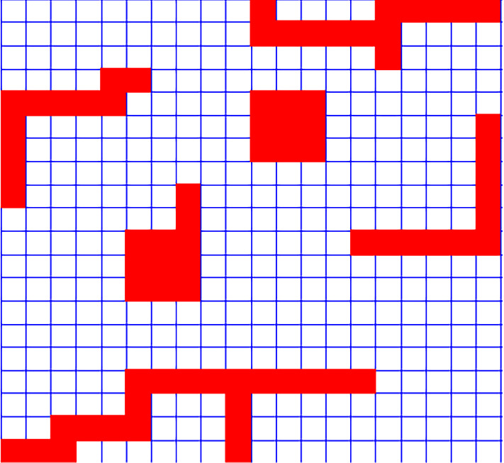
Study region with cluster area in red color. The shape of clusters is not circular (Color figure online)

Poisson Maps

In the first scenario, we generate the map with $20\times 20$ cells using Poisson distribution. The population of each cell is constant and set as 1000. We consider irregular shape clusters with different shapes in the map: (1) L shape, (2) circular, (3) circular with tail, (4) snake and (5) snake with two heads. These shapes are shown with red color in Fig. 2. Inside the red areas, we generate the number of cases using Poisson(12) and outside of those areas, using Poisson(10), which means a higher relative risk inside the cluster of $20\%$. Then, we apply three different algorithms, i.e., Ir-Poisson (Algorithm 1), Ir-binomial (Algorithm 2), and Ir-Bell (Algorithm 3) to detect clusters. We repeat this process 200 times. Using four criteria we compare the three algorithms. These criteria are biasness, recall, precision and harmonic mean of precision and recall (F1), which are as follows.

First, Prates et al. [36] discussed the relative risk and biasness in spatial scan statistics. The bias is defined as the true ratio of the parameters inside and outside the cluster to the ratio of their estimated value. Bias values near 1 mean that the selected clusters are better to estimate the relative risk between the cases inside and outside the clusters than detected clusters with a bigger or smaller value for biasness. The precision and recall are two famous criteria in clustering problems which are defined as:

$$\begin{array}{c}\hfill \text{Recall}={\displaystyle \frac{|\text{Detected cluster}\cap \text{True cluster}|}{|\text{True cluster}|}},\\ \hfill \text{Precision}={\displaystyle \frac{|\text{Detected cluster}\cap \text{True cluster}|}{|\text{Detected cluster}|}},\end{array}$$

and also

$$\begin{array}{c}\hfill F1={\displaystyle \frac{2(\text{recall}\times \text{precision})}{\text{recall+precision}}}\end{array}$$

such that |A| is the cardinality of set A.

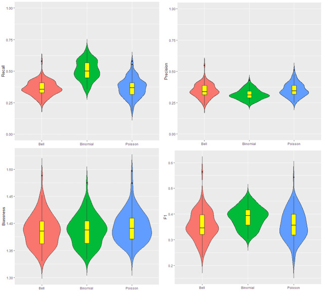
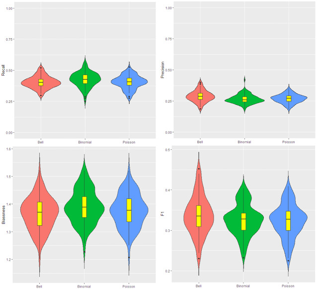
The results for this simulation are shown in Fig. 3. According to this figure, the recall for Ir-binomial is higher, but its precision is lower than the other scans. This means this model leads to over-estimation in cluster detection. The Ir-Poisson and Ir-Bell have very similar behavior in precision and recall. The bias values are almost the same for the three models. In the case of F1, Ir-Poisson and Ir-Bell are very similar and some times the F1 for them reaches to above 0.5, where Ir-binomial scan cannot reach that.

Fig. 3.

Data for the map are generated from the Poisson with parameter 12 and 10 respectively inside and outside cluster. From the top left to the bottom right: the violin plot for the recall, precision, bias, and F1. The number of iteration is 200. The red, green and blue colors are respectively for the Ir-Bell, Ir-binomial and Ir-Poisson scans (Color figure online)

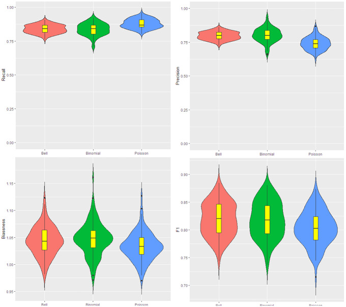
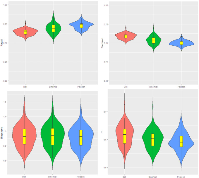
In the next step of the simulation, we change the parameter inside the cluster to 20 and consider the parameter outside cluster 10 providing a relative risk of 100%. The results of cluster detection are shown in Fig. 4. The recall (precision) for Ir-Poisson is higher (lower) than other scans. Since the recall for Ir-Poisson is near 1 and its precision is high, it means the true clusters are detected with few non-cluster areas also included as clusters. Ir-binomial has more bias, and the other scans are very similar to each other in this case. F1 for Ir-Bell and Ir-binomial are a little higher than Ir-Poisson.

Fig. 4.

Data for the map are generated from the Poisson with parameter 20 and 10, respectively, inside and outside cluster. From the top left to the bottom right: the violin plot for the recall, precision, bias, and F1. The number of iteration is 200. The red, green and blue colors are respectively for the Ir-Bell, Ir-binomial and Ir-Poisson scans (Color figure online)

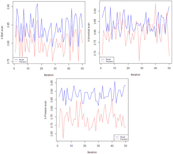
To have a better vision about the performance of three scans, we select the first 50 iterations of simulations and plot precision and recall point-wise in Fig. 5. Based on this figure, in the case of Ir-Poisson and Ir-Bell, precision is always under recall which is not true for Ir-binomial. Correlation of recall and precision for Ir-Bell, Ir-binomial, and Ir-Poisson are 1, $-0.17$, $-0.03$. This means we have more over-estimation and under-estimation in applying Ir-binomial. Considering these facts and the graph of bias value, we believe that Ir-Poisson and Ir-Bell detect clusters better in this scenario comparing to the Ir-binomial.

Fig. 5.

Variation of the recall and precision in the first 50 iteration of the simulation study for the scenario Poisson(10)-Poisson(20). The Ir-Bell, Ir-binomial and Ir-Poisson are presented

The increasing of the parameter inside the cluster from 20 to 40, causes recall, precision, bias, and F1 to become very close to 1, as expected because in this step the distinction between the cluster areas in comparison to the non-cluster areas is very large.

Binomial Maps

The results of cluster detection for binomial maps for different scenarios are presented and discussed in details in the Supplementary Material Section SM-3. Briefly, the Ir-Bell and Ir-binomial perform better in irregular shape cluster detection comparing to the Ir-Poisson scan.

Bell Maps

In the first step of this scenario, the cluster areas in the map are generated from a Bell($W_0(12)$). A Bell($W_0(10)$) is used to generate cases outside the cluster areas. Therfore, we guaratee a relative risk of $20\%$ inside the cluster. We apply three different scans (Ir-Bell, Ir-Poisson, Ir-binomial) to detect clusters. The results of comparison are presented in Fig. 6. We can see that the Ir-Bell scan outperforms the other methods under this scenario. Notice that F1 is much higher than the other two with a smaller bias.

Fig. 6.

Data for the map are generated from the Bell with parameter $W_0(12)$ and $W_0(10)$ respectively inside and outside cluster. From the top left to the bottom right: the violin plot for the recall, precision, bias, and F1 in 200 iteration. The red, green and blue colors are for the Ir-Bell, Ir-binomial and Ir-Poisson scans (Color figure online)

Increasing $W_0(12)$ to $W_0(20)$ leads us to declare that the Ir-Bell scan has better performance in cluster detection. Because bias values for this model are smaller than the two other models, and its F1 is higher. The results of the cluster detection are shown in Fig. 7. The three models have almost the same recall but the precision for Ir-Bell is considerably higher than the other two. This leads to high F1 and better bias value for the Ir-Bell scan. Finally, we increase the parameter inside the cluster to $W_0(40)$. In this case, the three scans have perfect performance and all criteria are close to 1.

Fig. 7.

Data for the map are generated from the Bell with parameter $W_0(20)$ and $W_0(10)$ respectively inside and outside cluster. From the top left to the bottom right: the violin plot for the recall, precision, bias, and F1. The number of iteration is 200. The red, green and blue colors are respectively for the Ir-Bell, Ir-binomial and Ir-Poisson scans (Color figure online)

Overall, we can conclude that the Ir-Bell scan is robust to other generation schemes (model misspecification) and outperform the other scans when is the true distribution. It is a strong candidate to consider when analysing real data.

Application

Irregularly Shaped Spatial Clusters in a Medical Image

In this section, a real data set is studied. Since we concluded in Sect. 4 that the Ir-Bell is a more robust scan statistics, we will proceed with our analysis using the Ir-Bell scan.

Any image can be considered as a map with many cells. Therefore, the scan statistic method was applied by Popescu and Lewitt [37] to detect circular small nodules on a medical image. We use the same image to detect small nodules with more details (irregular shape nodules) and compare the performance of our algorithm with their results. This image has $205\times 205=42,025$ pixels.

The location and the size of the true clusters are not known in practice. Hence, choosing the size of the scanning window in spatial clustering problems is a challenge for researchers. According to Kim and Jung [38], little research has been done on the maximum scan window size or maximum reported cluster size. Wang et al. [39] stated that the maximum window size effects on the size of detected clusters. According to their paper, historical information and information about the real cluster can help to determine the maximum size of the scanning window. For example, a researcher may be interested in finding small clusters (such as small cancerous glands), in which case it is recommended that the maximum size of the window be considered small. But, sometimes the goal of research is to find larger clusters, such as the clusters in the Covid-19 disease, which may even involve half of the population. In such cases, the researcher can consider the size of the scanning window to be large. Therefore, a suitable window size can be determined by the researcher’s prior information and experience.

Currently, the Gini coefficient and the maximum clustering set-proportion statistic (MCS-P) are the most common choices to select appropriate window size without any prior information [39]. Nevertheless, in our application we have prior information about the clusters [37], and since our goal is to provide algorithms for spatial cluster detection, we do not focus on the Gini coefficient to determine window size. Popescu and Lewitt [37] considered very small scan window size (about 0.5% of the image) such that the total detected area is about 10% of the total image because the detection of small nodules is the study objective.

The left side of Fig. 8 shows the circular scan window and the detected clusters. Our goal is to scan this image to find irregularly shaped clusters and compare the results with the result of Popescu and Lewitt [37]. We use the proposed Ir-Bell, Ir-Binomial, and Ir-Poisson scan algorithms and consider the maximum size window varying from 1%, 5%, and 10% of the image. As previously mentioned, the location and size of the correct clusters are unknown in real data. On the other hand, the maximum scanning window size affects clustering results. Based on the results of Popescu and Lewitt [37], we choose equal window sizes. These choices have the following advantages: scanning by 1% determines the center of the cluster, in other words, where a nodule starts to grow. Scanning by 5% and 10% helps us to see whether increasing the window size has a significant effect on cluster detection or not. The significant difference can be examined through eye comparisons. As we can see, there is no significant difference between the latter two results. It is worth noting that the method of Popescu and Lewitt [37] has at least two disadvantages: first, it detects clusters in a circular shape, and second, as can be seen in Fig. 8 (left side), the radius of blue circles are equal. It is expected that the size of cancerous glands in the body does not have such restriction, as can be seen in the other windows of Fig. 8.

Fig. 8.

From the left to the right: (1) detection of circular small nodules in a medical image by Popescu and Lewitt [37]. (2), (3) and (4): Detection of small irregular shape nodules in a medical image by the Ir-Bell scan statistic using, respectively, 1%, 5% and 10% of total image as window size

The results of cluster detection in the medical image are in Fig. 8 for Ir-Bell scan. The regions of detected clusters by the Ir-Bell scan algorithm are very similar to the locations of the clusters detected by Popescu and Lewitt [37]. However, our algorithm is capable of providing more details in the shape of the clusters, avoiding over or under detection of the clusters areas. It should be noted that by applying Ir-Binomial and Ir-Poisson scans, similar results are obtained. In Fig. 9, a part of the image is selected and magnified to see the same performance of Ir-Bell, Ir-Poisson, and Ir-Binomial more clearly. They perform equally for different scanning methods.

Fig. 9.

From the left to the right: (1) Irregular shape clusters detected by the Ir-Bell model based on Monte-Carlo. (2) Irregular shape clusters detected by the Ir-Binomial model based on Monte-Carlo and without it. (3) Irregular shape clusters detected by the Ir-Poisson model with and without Monte-Carlo. The explored area is $50\times 50$ pixels on the top left of medical image

Execution Time for New Algorithms

According to Zhou et al. [25], 20, 000 random data sets are needed to find irregular shape clusters based on Monte-Carlo hypothesis testing. The scan process for this number of data sets is troublesome when the map is big. Hence the elimination of Monte-Carlo from irregular shape cluster detection can decrease detection time making the methodology better prepared for the real-life challenges of nowadays.

Algorithms 1 and 2 (Ir-Poisson and Ir-binomial respectively) in our paper are independent of the Monte-Carlo method. Therefore, we can compare the execution time to detect irregular shape clusters with and without Monte-Carlo hypothesis testing.

To this aim, we select just $50\times 50$ pixels in the top left of the medical image. This partial area is selected because the traditional algorithms require 20, 000 iterations of Monte-Carlo and this study would be time-consuming for the whole image with 42, 025 pixels. The detected clusters by the different methods are shown in Fig. 9. As expected, all models return the same clusters for the fast and slow versions. Unlike Popescu and Lewitt [37], we do not have access to a cluster of high computational performance. Instead, we used our R [40] coding in a desktop computer core i5 with 4Gb of RAM and Windows 7. Under such a configuration, the Ir-Bell method takes about 8 h to scan the entire image.

The execution times and p values are in Table 1. First, it is important to emphasize that the p values returned by Monte-Carlo and theoretical are the same. Also, this table reveals the advantage of the elimination of the Monte-Carlo procedure in decreasing detection time which is decreased by an order of $50\%$. All of our codes are performed in R and more improvement can be done in the execution time if a better implementation of the methods is explored.

Table 1.

Execution time in minutes for detecting spatial clusters with and without the Monte-Carlo procedure

	Bell	Binomial	Poisson
With Monte-Carlo	30.41	43.28	36.62
Without Monte-Carlo	–	17.44	16.01
p-value	$<0.0002$	$<0.0002$	$<0.0002$

Conclusion

In this paper, we introduce new approaches to handle big maps in spatial clustering problems. To do this, three scan statistics are presented: Ir-Poisson scan, Ir-binomial scan (Sect. 3.1), and Ir-Bell scan (Sect. 3.2).

By our simulation studies, we show that the Ir-Bell scan statistic outperforms the traditional Poisson and binomial scan statistics in cluster detection when it is the true distribution.

We apply our methods to a medical image. The results verify the results of Popescu and Lewitt [37], however, provide more insights and richness in terms of interpretation, since the shape of the detect cluster are more precise. Moreover, using our naive R implementation, we show that, with the same results, the fast scan versions of the Ir-Poisson and Ir-binomial (Algorithms 1 and 2) perform at least two times faster than the traditional ones that rely on Monte-Carlo simulation.

Finally, as future work, we are interested in studying and extending these irregular shape cluster detection to their zero-inflated fast versions. Nowadays it is common to have data sets that are zero-inflated. Thus, zero-inflated methods have become relevant to provide more realistic, precise, and adequate analysis for the data.

Supplementary Information

Below is the link to the electronic supplementary material.

References

- 1.Adelberger KL, Steidel CC, Pettini M, Shapley AE, Reddy NA, Erb DK. The spatial clustering of star-forming galaxies at redshifts 1.4 3.5. Astrophys J. 2005;619(2):697. doi: 10.1086/426580. [DOI] [Google Scholar]
- 2.Mo H, White SD. An analytic model for the spatial clustering of dark matter haloes. Mon Not R Astron Soc. 1996;282(2):347–361. doi: 10.1093/mnras/282.2.347. [DOI] [Google Scholar]
- 3.Haralick R, Dinstein I. A spatial clustering procedure for multi-image data. IEEE Trans Circuits Syst. 1975;22(5):440–450. doi: 10.1109/TCS.1975.1084059. [DOI] [Google Scholar]
- 4.Zhang L, Zhu Z (2012) Spatial multiresolution cluster detection method. arXiv:1205.2106
- 5.Han J (2001) Spatial clustering methods in data mining: a survey. Geographic data mining and knowledge discovery, pp 188–217
- 6.Harries KD et al (1999) Mapping crime: principle and practice. Technical report, US Department of Justice, Office of Justice Programs, National Institute of Justice
- 7.Murray AT, Grubesic TH, Wei R. Spatially significant cluster detection. Spat Stat. 2014;10:103–116. doi: 10.1016/j.spasta.2014.03.001. [DOI] [Google Scholar]
- 8.Myers N, Mittermeier RA, Mittermeier CG, Da Fonseca GA, Kent J. Biodiversity hotspots for conservation priorities. Nature. 2000;403(6772):853. doi: 10.1038/35002501. [DOI] [PubMed] [Google Scholar]
- 9.Stohlgren TJ, Binkley D, Chong GW, Kalkhan MA, Schell LD, Bull KA, Otsuki Y, Newman G, Bashkin M, Son Y. Exotic plant species invade hot spots of native plant diversity. Ecol Monogr. 1999;69(1):25–46. doi: 10.1890/0012-9615(1999)069[0025:EPSIHS]2.0.CO;2. [DOI] [Google Scholar]
- 10.Grubesic TH. On the application of fuzzy clustering for crime hot spot detection. J Quant Criminol. 2006;22(1):77. doi: 10.1007/s10940-005-9003-6. [DOI] [Google Scholar]
- 11.Yamada I, Rogerson P. Statistical detection and surveillance of geographic clusters. Boca Raton: Chapman and Hall/CRC; 2008. [Google Scholar]
- 12.Haralick R, Kelly G. Pattern recognition with measurement space and spatial clustering for multiple images. Proc IEEE. 1969;57(4):654–665. doi: 10.1109/PROC.1969.7020. [DOI] [Google Scholar]
- 13.Gutteridge A, Bartlett GJ, Thornton JM. Using a neural network and spatial clustering to predict the location of active sites in enzymes. J Mol Biol. 2003;330(4):719–734. doi: 10.1016/S0022-2836(03)00515-1. [DOI] [PubMed] [Google Scholar]
- 14.Bar-Hen A, Emily M, Picard N. Spatial cluster detection using nearest neighbor distance. Spat stat. 2015;14:400–411. doi: 10.1016/j.spasta.2015.07.006. [DOI] [Google Scholar]
- 15.Culvenor DS, Coops N, Preston R, Tolhurst KG (1998) A spatial clustering approach to automated tree crown delineation. In: Proceedings of the international forum on automated interpretation of high spatial resolution digital imagery for forestry, pp 67–80
- 16.Duczmal LH, Moreira GJ, Burgarelli D, Takahashi RH, Magalhães FC, Bodevan EC. Voronoi distance based prospective space-time scans for point data sets: a dengue fever cluster analysis in a southeast Brazilian town. Int J Health Geogr. 2011;10(1):29. doi: 10.1186/1476-072X-10-29. [DOI] [PMC free article] [PubMed] [Google Scholar]
- 17.Wieland SC, Brownstein JS, Berger B, Mandl KD. Density-equalizing euclidean minimum spanning trees for the detection of all disease cluster shapes. Proc Natl Acad Sci. 2007;104(22):9404–9409. doi: 10.1073/pnas.0609457104. [DOI] [PMC free article] [PubMed] [Google Scholar]
- 18.Kulldorff M, Nagarwalla N. Spatial disease clusters: detection and inference. Stat Med. 1995;14(8):799–810. doi: 10.1002/sim.4780140809. [DOI] [PubMed] [Google Scholar]
- 19.Kulldorff M. A spatial scan statistic. Commun Stat Theory Methods. 1997;26(6):1481–1496. doi: 10.1080/03610929708831995. [DOI] [Google Scholar]
- 20.Cançado AL, da Silva CQ, da Silva MF. A spatial scan statistic for zero-inflated poisson process. Environ Ecol Stat. 2014;21(4):627–650. doi: 10.1007/s10651-013-0272-1. [DOI] [Google Scholar]
- 21.Abolhassani A, Prates MO, Castellares F, Mahmoodi S. Zero-inflated bell scan: a more flexible spatial scan statistic. Spat Stat. 2020;36:100433. doi: 10.1016/j.spasta.2020.100433. [DOI] [Google Scholar]
- 22.de Lima MS, Duczmal LH, Neto JC, Pinto LP. Spatial scan statistics for models with overdispersion and inflated zeros. Stat Sin. 2015;25:225–241. [Google Scholar]
- 23.Assunção R, Costa M, Tavares A, Ferreira S. Fast detection of arbitrarily shaped disease clusters. Stat Med. 2006;25(5):723–742. doi: 10.1002/sim.2411. [DOI] [PubMed] [Google Scholar]
- 24.Costa MA, Assunção RM, Kulldorff M. Constrained spanning tree algorithms for irregularly-shaped spatial clustering. Comput Stat Data Anal. 2012;56(6):1771–1783. doi: 10.1016/j.csda.2011.11.001. [DOI] [Google Scholar]
- 25.Zhou R, Shu L, Su Y. An adaptive minimum spanning tree test for detecting irregularly-shaped spatial clusters. Comput Stat Data Anal. 2015;89:134–146. doi: 10.1016/j.csda.2015.03.008. [DOI] [Google Scholar]
- 26.Yin P, Mu L. A hybrid method for fast detection of spatial disease clusters in irregular shapes. GeoJournal. 2018;83(4):693–705. doi: 10.1007/s10708-017-9799-2. [DOI] [Google Scholar]
- 27.Abolhassani A, Prates MO. An up-to-date review of scan statistics. Stat Surv. 2021;15:111–153. doi: 10.1214/21-SS132. [DOI] [Google Scholar]
- 28.Castellares F, Prates MO, Abolhassani A. Comments on “a spatial scan statistic for compound poisson data”. Stat Med. 2019;38(7):1297–1299. doi: 10.1002/sim.8006. [DOI] [PubMed] [Google Scholar]
- 29.Kulldorff M, Huang L, Pickle L, Duczmal L. An elliptic spatial scan statistic. Stat Med. 2006;25(22):3929–3943. doi: 10.1002/sim.2490. [DOI] [PubMed] [Google Scholar]
- 30.Neill DB. Fast subset scan for spatial pattern detection. J R Stat Soc Ser B. 2012;74(2):337–360. doi: 10.1111/j.1467-9868.2011.01014.x. [DOI] [Google Scholar]
- 31.Aboukhamseen S, Soltani A, Najafi M. Modelling cluster detection in spatial scan statistics: formation of a spatial poisson scanning window and an adhd case study. Stat Probab Lett. 2016;111:26–31. doi: 10.1016/j.spl.2015.12.025. [DOI] [Google Scholar]
- 32.Soltani A, Aboukhamseen S. An alternative cluster detection test in spatial scan statistics. Commun Stat Theory Methods. 2015;44(8):1592–1601. doi: 10.1080/03610926.2013.777740. [DOI] [Google Scholar]
- 33.Prim RC. Shortest connection networks and some generalizations. Bell Syst Tech J. 1957;36(6):1389–1401. doi: 10.1002/j.1538-7305.1957.tb01515.x. [DOI] [Google Scholar]
- 34.Bell ET. Exponential numbers. Am Math Mon. 1934;41(7):411–419. doi: 10.1080/00029890.1934.11987615. [DOI] [Google Scholar]
- 35.Bell ET. Exponential polynomials. Ann Math. 1934;35(2):258–277. doi: 10.2307/1968431. [DOI] [Google Scholar]
- 36.Prates MO, Kulldorff M, Assunção RM. Relative risk estimates from spatial and space-time scan statistics: are they biased? Stat Med. 2014;33(15):2634–2644. doi: 10.1002/sim.6143. [DOI] [PMC free article] [PubMed] [Google Scholar]
- 37.Popescu LM, Lewitt RM. Small nodule detectability evaluation using a generalized scan-statistic model. Phys Med Biol. 2006;51(23):6225. doi: 10.1088/0031-9155/51/23/020. [DOI] [PubMed] [Google Scholar]
- 38.Kim S, Jung I. Optimizing the maximum reported cluster size in the spatial scan statistic for ordinal data. PLoS ONE. 2017;12(7):e0182234. doi: 10.1371/journal.pone.0182234. [DOI] [PMC free article] [PubMed] [Google Scholar]
- 39.Wang W, Zhang T, Yin F, Xiao X, Chen S, Zhang X, Li X, Ma Y. Using the maximum clustering heterogeneous set-proportion to select the maximum window size for the spatial scan statistic. Sci Rep. 2020;10(1):1–14. doi: 10.1038/s41598-020-61829-y. [DOI] [PMC free article] [PubMed] [Google Scholar]
- 40.R Core Team (2019) R: a language and environment for statistical computing. R Foundation for Statistical Computing, Vienna, Austria
Associated Data
This section collects any data citations, data availability statements, or supplementary materials included in this article.