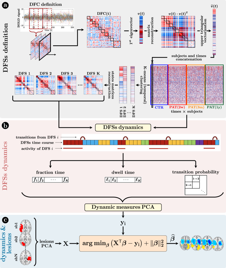
Fig. 1. Methods (dynamical functional states).

a Definition of the dynamic functional states (DFSs): (i) at first, the time course of each subject was divided into 270 time-windows of width = 30 TR (600 s) and step = 1 TR. The z-Fisher transform of the Pearson’s correlation coefficient among regions was computed at each sliding window, to estimate the Dynamical Functional Connectivity (DFC). Then, (ii) each DFC matrix was approximated by projecting on the leading eigenspace defined by the first eigenvector $v_i$. As the eigenvectors are defined less than the sign, we avoided this issue by reconstructing the square matrix $v_i\times v_i^T$. After that, (iii) the upper triangular part of these rank-one DFC matrices was vectorized and concatenated across windows and subjects, in order to finally apply a time-wise K-means clustering algorithm with correlation distance and 20 replicates (iv) to define a set of K spatial DFSs. Silhouette and Davies-Bouldin algorithms were used to search for the optimal number of DFSs. Several choices of K (from 2 to 10) were used for supplementary analyses and comparisons. b The K-means clustering associated each sliding window to a specific DFS, thus for each subject we obtained a discrete time series $x\left(n\right)$, with n = 1,…, 270, where each discrete value (between 1 and K) indicated the active state at that time point. From these time courses it was possible to evaluate three different dynamical measures for each state, namely the fraction time, the dwell time, and the transition probability. To analyze the relationship among dynamical measures in healthy condition, we performed a Principal Component Analysis (PCA) over all the dynamical measures. c The projection of the sub-acute patients’ dynamical measures onto the PCs space, and the anatomical brains lesions were used as input for a Ridge Regression algorithm, aimed at identifying the lesion’s location that better characterized specific dynamic impairments. A similar approach has been used with structural disconnections.