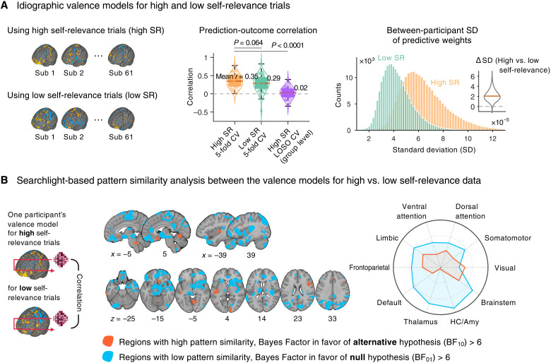
Fig. 6. Idiographic predictive modeling of valence.

(A) We used an idiographic predictive modeling approach to quantifying the between-participant variability of predictive weights for high versus low self-relevance data. We trained two valence models per person—the first model used data from the trials with the high self-relevance scores (>0.5; high SR) and the other used data from the trials with low self-relevance scores (≤0.5; low SR). In addition, we trained a group-level valence model by concatenating all participants’ high self-relevance data with LOSO-CV for comparison. The violin and box plots in the middle show the prediction performance of two idiographic models with 5-fold cross-validation and the group-level model with LOSO-CV. Each dot represents each participant. The histograms on the right show the distributions of the between-participant SD of predictive weights, and the inset violin plot shows the differences in the SD between two valence models across voxels. (B) We examined which brain regions displayed similar or distinct spatial patterns of predictive weights between two valence models with a searchlight-based pattern similarity analysis. For this, we first created a searchlight with a radius of five voxels and scanned it throughout the whole brain with a step size of four voxels. We then calculated correlation coefficients between the two models’ predictive weights within each searchlight. The red regions showed Bayes factor values in favor of having distinct patterns between two models (BF₁₀ > 6), whereas the blue regions were the opposite, i.e., in favor of having similar patterns (BF₀₁ > 6). The radial plot shows the relative proportions of overlapping voxels between the thresholded map and large-scale networks, given the total number of voxels within each network.