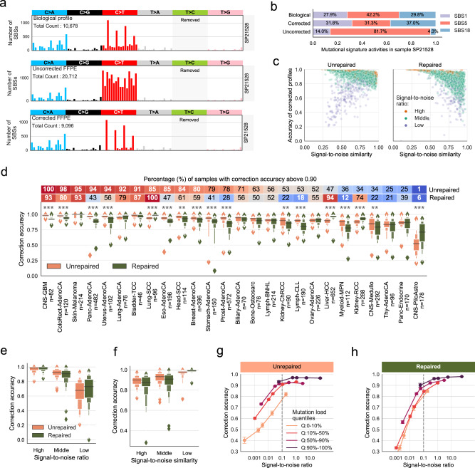
Fig. 2. Correction of FFPE artefacts in synthetic FFPE samples using FFPEsig.

a The correction result for one CRC sample as an example. b Similar activities resulted from the corrected profile compared to the true biological profile for the CRC sample in a. c Correction accuracy for all synthetic FFPE samples. We grouped n = 2780 samples into three categories according to biological C>T mutation count: high (top 10%, n = 278), low (bottom 10%, n = 278) and middle (the remaining 80%, n = 2224). d Correction accuracy varied among cancer types. The percentage of samples with accuracy >0.90 is annotated in the heatmap bar. Data are presented using a Letter-Value plot and the black line corresponds to the median of the dataset and every further step splits the remaining data into two halves (the same for e, f below). The statistical difference between repaired versus unrepaired FFPEs is derived from the two-sided Mann–Whitney U test. P ≤ 0.001 (***); P ≤ 0.01 (**); P ≤ 0.05 (*). e Positive correlation between signal-to-noise ratio and correction accuracy. We classified all samples based on SNR into three groups: high (top 10%, n = 278), low (n = 278, bottom 10%) and middle (the remaining 80%, n = 2224). f Negative correlation between signal-to-noise similarity and correction accuracy. Unrepaired: n = 278 (high), n = 2023 (middle) and n = 201 (low) samples. Repaired: n = 244 (high), n = 1984 (middle) and n = 274 (low) samples. g, h FFPEsig works well in samples with SNR above 0.1 for both unrepaired (g) and repaired (h) FFPEs. We generated five sets (n = 2780 per set) synthetic samples by adding increasing noise (10³, 10⁴, 5 × 10⁴, 10⁵ to 10⁶) to PCAWG samples. We divided samples in each set into four categories depending on biological C>T mutation load (from the lowest to the highest): Q:0–10% (n = 278), Q:10–50% (n = 1112), Q:50–90% (n = 1112) and Q:90–100% (n = 278). Data are presented as mean values within each category ± 95% confidence interval. All statistics are derived from biological independent samples.