Insights from the IronTract challenge: Optimal methods for mapping brain pathways from multi-shell diffusion MRI

Abstract

Limitations in the accuracy of brain pathways reconstructed by diffusion MRI (dMRI) tractography have received considerable attention. While the technical advances spearheaded by the Human Connectome Project (HCP) led to significant improvements in dMRI data quality, it remains unclear how these data should be analyzed to maximize tractography accuracy. Over a period of two years, we have engaged the dMRI community in the IronTract Challenge, which aims to answer this question by leveraging a unique dataset. Macaque brains that have received both tracer injections and ex vivo dMRI at high spatial and angular resolution allow a comprehensive, quantitative assessment of tractography accuracy on state-of-the-art dMRI acquisition schemes. We find that, when analysis methods are carefully optimized, the HCP scheme can achieve similar accuracy as a more time-consuming, Cartesian-grid scheme. Importantly, we show that simple pre- and post-processing strategies can improve the accuracy and robustness of many tractography methods. Finally, we find that fiber configurations that go beyond crossing (e.g., fanning, branching) are the most challenging for tractography. The IronTract Challenge remains open and we hope that it can serve as a valuable validation tool for both users and developers of dMRI analysis methods.

1. Introduction

Diffusion MRI (dMRI) tractography allows us to image brain pathways in vivo and non-invasively, and is thus a useful tool in a variety of research and clinical settings. However, it relies on indirect measurements of axonal orientations extracted from the dMRI signal, which can lead to errors in the reconstructed pathways. Possible sources of these errors, as identified by early studies, included uncertainty in the signal due to imaging noise (Jones, 2003) and crossing fibers (Tuch et al., 2003). These issues motivated the effort to improve the signal-to-noise ratio (SNR), as well as the spatial and angular resolution of dMRI. The Human Connectome Project (HCP) sought to address these needs by developing scanners with ultra-high gradients, which allowed higher b-values to be acquired without sacrificing SNR, and accelerated dMRI sequences, which enabled higher angular and spatial resolution with shorter acquisition times (Harms et al., 2018; Setsompop et al., 2013; Sotiropoulos et al., 2013; Van Essen et al., 2013). These developments made multi-shell dMRI data prevalent. In parallel, orientation reconstruction methods were adapted to make better use of such data (Aganj et al., 2010; Canales-Rodríguez et al., 2009; Christiaens et al., 2015; Jbabdi et al., 2012; Jeurissen et al., 2014).

These advances in data acquisition and analysis improved our ability to resolve crossing fibers within a voxel (Fan et al., 2014; Jones et al., 2018) and allowed us to reconstruct white-matter circuitry in greater detail than previously possible (Edlow et al., 2016; Maffei et al., 2018). However, it is unclear which analysis methods maximize the anatomic accuracy of the pathways that can be reconstructed from these state-of-the-art acquisition protocols. Given the large amounts of HCP-style, multi-shell data that are now publicly available (Bookheimer et al., 2019; Casey et al., 2018; Harms et al., 2018; Van Essen et al., 2013), and the plethora of methods for pre-processing, orientation reconstruction, and tractography that can be applied to these data, it is of critical importance to compare these methods with respect to objective metrics of anatomic accuracy.

Anatomic tracing in non-human primates (NHPs) can be used to assess the accuracy of tractography in the brain (Yendiki et al., 2021). It allows us to reconstruct the complete trajectories of axon bundles from a tracer injection site to their destinations throughout the brain. The majority of previous studies that compared dMRI tractography to anatomic tracing were limited to single-shell dMRI data (Azadbakht et al., 2015; Dauguet et al., 2007; Gao et al., 2013; Schilling et al., 2019a; Schilling et al., 2019b; Thomas et al., 2014; van den Heuvel et al., 2015). Furthermore, the majority of such studies only considered the end points of the fiber bundles, and not their complete trajectory (Ambrosen et al., 2020; Azadbakht et al., 2015; Donahue et al., 2016; Girard et al., 2020; Hagmann et al., 2008; van den Heuvel et al., 2015). That is because they did not have dMRI and tracer data from the same brains, hence they relied on connectivity matrices from existing tracer databases.

The IronTract Challenge is the first open tractography challenge to be conducted on high-resolution, densely sampled brain dMRI data. This allowed us to evaluate tractography accuracy for two widely adopted sampling schemes: multi-shell and Cartesian-grid. We leveraged a unique collection of NHP brains, where both anatomic tracer injections and ex vivo dMRI had been performed (Grisot et al., 2021; Safadi et al., 2018; Tang et al., 2019). The availability of dMRI and tracer data in the same brains allowed us to evaluate the accuracy of tractography not only at the end points of the axon bundles but along their trajectory in the white matter. This is the only way to localize exactly where tractography algorithms go wrong, which is a necessary step towards determining why they go wrong, and therefore how to improve them.

The IronTract Challenge also differed from previous tractography challenges in terms of its design. Participants submitted results with a wide range of tractography thresholds. When methods are compared only at their default thresholds (e.g., (Maier-Hein et al., 2017; Schilling et al., 2019a; Thomas et al., 2014)), they differ in terms of both sensitivity and specificity, and it is impossible to disentangle the effect of the threshold and the effect of the algorithm. Our design allowed us to circumvent this issue and to compare algorithms in terms of their sensitivity at the same level of specificity.

A previous validation study used data only from the training case of this challenge and performed a systematic comparison of a small number of q-space sampling, orientation reconstruction, and tractography methods, in all their permutations (Grisot et al., 2021). The IronTract Challenge expands the scope of our prior validation studies in two major ways. First, challenge participants chose a much wider range of state-of-the-art orientation reconstruction and tractography methods. Second, the addition of the validation case, which involved an injection in a different anatomical location and fibers following very different trajectories than the training case, allowed us to compare the robustness of the methods to the location of the seed region.

The IronTract Challenge was administered in two rounds (https://irontract.mgh.harvard.edu). The first round was organized in the context of the 2019 international conference on Medical Image Computing and Computer-Assisted Intervention. Preliminary results from the first and second rounds were presented, respectively, at the 2020 and 2021 annual meetings of the International Society for Magnetic Resonance in Medicine (Maffei et al., 2021, 2020). In the first round, two teams outperformed all others, achieving both high accuracy and robustness to the location of the seed region. This motivated the second round, where all participants revisited their analyses, replacing their pre- and post-processing steps with those of the two high-performing teams. This allowed us to investigate the extent to which performance was dependent on the pre- and post-processing vs. the orientation reconstruction and tractography methods. The outcomes of this effort, as detailed below, include (i) practical recommendations for users of HCP-style, multi-shell dMRI data, who are interested in methods for analyzing these data that maximize anatomical accuracy, and (ii) insights on the fundamental failure modes of tractography for method developers, who are interested in potential avenues for improving these methods.

2. Methods

2.1. Outline of the challenge

Both rounds of the IronTract challenge followed the outline shown in Fig. 1. In vivo tracer injections and ex vivo dMRI scanning were performed on two macaque brains (see 2.2 Data description). The dMRI data, acquired on a Cartesian grid, were resampled onto the two-shell of the HCP acquisition protocol (Harms et al., 2018). We will refer to these datasets as diffusion spectrum imaging (DSI) and HCP respectively. The organizing team uploaded the data to the QMENTA platform (https://qmenta.com/irontract-challenge/) and the challenge teams could download them along with the tracer injection sites in the dMRI space. Each team analyzed the data with methods of their choice (see 2.3 Analysis of dMRI data by challenge participants). In round 1, this included image pre-processing, orientation reconstruction, tractography, and tractogram post-processing. In round 2, the pre- and post-processing steps were standardized across all teams. Each team produced tractograms with a range of thresholds and uploaded them to the QMENTA platform. A score was computed on the fly by comparing the tractograms to the tracer data (see 2.4 ROC analysis). For the training case, participants were shown their score and were allowed to repeat data analysis and upload of results. Thus, participants tuned their analysis pipelines to maximize their score on the training case. Finally, they applied the optimized pipeline to the data from the validation case. The organizing team computed AUC scores on the validation case and used them for the final ranking of the challenge teams.

Fig. 1. Overview of the IronTract Challenge.

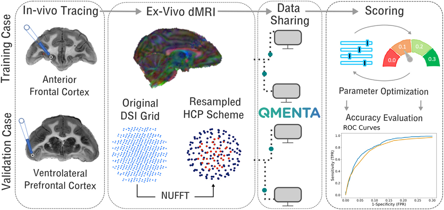
Data from two monkey brains, one with an injection in the anterior frontal cortex and one with an injection in the vlPFC, served as the training and validation case, respectively. Ex vivo dMRI data were acquired for both brains on a Cartesian grid (515 directions, bmax = 40, 000 s/mm²) and resampled via NUFFT on the two shells of the HCP lifespan acquisition scheme, with b-values adjusted for ex vivo dMRI (93 directions with b = 6000 s/mm², 92 directions with b = 12, 000 s/mm²). Participants downloaded data and uploaded results on the QMENTA platform. For the training case, they received a score, allowing them to optimize their tractography pipeline. The optimized pipelines were then applied to the validation case for the final scores.

2.2. Data description

The training and validation cases used in this challenge are part of a previously described dataset that consists of in vivo tracing and high-resolution ex vivo dMRI acquired in the same macaque brains (Grisot et al., 2021; Safadi et al., 2018; Tang et al., 2019).

2.2.1. Tracer injections

The training and validation datasets came from two different male rhesus macaques. The former received an injection of the anterograde/bidirectional tracer Lucifer Yellow in the anterior frontal cortex (frontal pole). The latter received an injection of the anterograde/bidirectional tracer Fluorescein in the ventrolateral prefrontal cortex (vlPFC). Surgery and tissue preparation were performed at the University of Rochester Medical Center. Details of these procedures were described previously (Haber, 1988; Lehman et al., 2011; Safadi et al., 2018). Briefly, each monkey received an injection of a bidirectional tracer conjugated with dextran amine (40–50 nl, 10% in 0.1 M phosphate buffer, pH 7.4; Invitrogen). Twelve days after the injection, animals were perfused and their brains were postfixed overnight and cryoprotected in increasing gradients of sucrose (10, 20, and 30%). All experiments were performed in accordance with the Institute of Laboratory Animal Resources Guide for the Care and Use of Laboratory Animals and approved by the University of Rochester Committee on Animal Resources.

2.2.2. dMRI data acquisition

After fixation, the brains were scanned in a small-bore 4.7T Bruker BioSpin scanner (maximum gradient strength 480 mT/m) using a 3D EPI sequence with the following parameters: T R = 750 ms, T E = 43 ms, δ = 15 ms, Δ = 19 ms, maximum b = 40, 000 ss/mm², matrix size 96 × 96 × 112, 0.7 mm isotropic resolution. Brains were submerged in liquid Fomblin to eliminate susceptibility artifacts. We acquired 1 non-diffusion weighted (b = 0 s/mm²) volume and 514 diffusion-weighted volumes corresponding to a Cartesian lattice in q-space. The total acquisition time was 48 h. We refer to this q-space sampling scheme data as DSI.

We resampled the data onto q-shells, following a methodology that was previously described and validated (Jones et al., 2021, 2020). It involves approximating data points distributed on spheres in q-space from data points distributed on a Cartesian grid, using a fast implementation of the non-uniform fast Fourier transform (NUFFT) (Fessler and Sutton, 2003). We followed this procedure to generate data on the two q-shells of the lifespan and disease HCP acquisition protocol (Harms et al., 2018). This in vivo protocol includes 93 directions with b = 1, 500 s/mm² and 92 directions with 3, 000 s/mm^2.We multiplied these b-values by the 4x factor required to achieve comparable diffusion contrast ex vivo as in vivo (Dyrby et al., 2011), i.e., we used b = 6000 and 12000 s/mm². We refer to this q-space sampling scheme as HCP.

To assess the SNR, we first fit the tensor model to the data and then delineated a mask encompassing the CC by selecting the highly red voxels in the color-coded fractional anisotropy (FA) map. We extracted the mean signal from this mask and from a mask outside the brain to capture the noise. We computed the SNR as the mean (signal)/standard deviation (noise) (Jones et al., 2013) for the b = 0 image (training: 63.56, validation: 51.16) and a for a b = 40,000 s/mm² image (training: 16.42, validation: 12.76). The computation was done in DIPY (Garyfallidis et al., 2014).

2.2.3. Histological processing

Following whole-brain ex vivo dMRI, the brains were returned to the University of Rochester for histological processing. They were sectioned in 50 μm thick coronal slices on a freezing microtome into 0.1 m phosphate buffer or cryoprotectant solution as previously described (Haber et al., 2000). An undistorted photo of the blockface was taken before cutting for use in image registration (See 2.2.4 Registration of tracer and dMRI data). Immunocytochemistry was then performed on every 8th slice to visualize the transported tracer, resulting in an inter-slice resolution of 400 μm. Additional details on the histological procedures can be found elsewhere (Haber et al., 2006; Haynes and Haber, 2013; Lehman et al., 2011). Labeled fiber bundles were outlined under dark-field illumination with a 4.0 or 6.4x objective, using Neurolucida software (MBF Bioscience). Fibers traveling together were outlined as a group or bundle. Axons were charted as they left the tracer injection site and followed through the right hemisphere, until the anterior commissure. The 2D outlines were combined across slices using IMOD software (Boulder Laboratory (Kremer et al., 1996)) to create 3D renderings of the structures and pathways as they traveled through them. These 2D outlines were used to further refine bundle contours and ensure spatial consistency across sections.

2.2.4. Registration of tracer and dMRI data

Each histology slice was registered to its corresponding blockface using a 2D robust affine registration (Reuter et al., 2010), followed by a 2D symmetric diffeomorphic registration (Avants et al., 2008). Blockface images were then stacked to create a 3D volume and registered to the b=0 dMRI volume using a 3D affine registration followed by a 3D diffeomorphic registration, with the same methods as above. The computed transformations were then applied to the tracer mask and the injection site mask, to map them into dMRI space. The transformed injection site mask was shared with challenge participants, to be used as the seed region for tractography.

2.3. Analysis of dMRI data by challenge participants

2.3.1. Round 1

In the first round, teams were provided raw dMRI data. They were allowed to use the q-space sampling scheme and analysis methods of their choice. A detailed description of the methods that each team used in this round, including pre-processing, orientation reconstruction method, tractography, and post-processing, are provided in the Supplementary note 1. Both probabilistic and deterministic tractography approaches were deployed, with a variety of orientation reconstruction methods. Participants were asked to generate tractograms at multiple thresholds by varying one or more parameters of their choice. The most common choices were lower thresholds on probability, for submissions that used a probabilistic tractography algorithm; and upper thresholds on the bending angle, sometimes combined with lower thresholds on fractional anisotropy or other microstructural parameters, for submissions that used a deterministic tractography algorithm.

For each submission, participants uploaded a series of volumes, obtained by applying different thresholds to the tractograms, to the QMENTA platform. A score was computed on the fly by comparing the tractograms to the tracer data (see 2.4 ROC analysis). For the training case, the platform generated a performance report, including the AUC score, and made it available to the participant. Participants could repeat their analysis, upload, and score any number of times, allowing them to fine-tune the free parameters of their methods and optimize their score. They then applied their optimized analysis pipeline to the dMRI data from the validation case and uploaded the resulting tractograms to the QMENTA platform.

2.3.2. Round 2

In the second round, analysis and scoring of the training and validation cases were performed as described above. The difference was that the pre- and post-processing steps were standardized across teams. Participants downloaded pre-processed dMRI data from the QMENTA platform and were provided two scripts for the post-processing steps. The orientation reconstruction and tractography methods were not standardized.

Pre-processing:

This followed the dMRI pre-processing procedures that had been used in round 1 by Team 1, the team that achieved the best performance (see 3.1 Round 1 Results). They included denoising (Veraart et al., 2016) and correction for Gibbs ringing (Kellner et al., 2016) in MRtrix3 (Tournier et al., 2019), and correction for motion and eddy-current distortions in FSL (Andersson et al., 2003; Andersson and Sotiropoulos, 2015). A binary dilation was applied to the tracer injection site mask.

Orientation reconstruction and tractography:

Teams were asked to apply the same orientation reconstruction and tractography methods as in round 1, if they had participated in round 1, or any methods of their choice otherwise. Supplementary note 2 details the orientation reconstruction and tractography method used by the teams in round 2.

Post-processing:

This replicated the post-processing strategies that had been used by the two teams that had consistently good performance across both training and validation cases in round 1. (i) Gaussian filtering. This strategy had been implemented by Team 1 in round 1. It included the application of a Gaussian filter with sigma = 0.5 to increase coverage, followed by an iterative thresholding of 200 steps on the log of the streamline count, for a total of 200 output tractogram volumes. (ii) Anatomical ROIs. This strategy had been implemented by Team 2 in round 1. ROIs from the PennCHOP macaque atlas (Feng et al., 2017) were transformed to the space of each dMRI dataset. Only streamlines intersecting at least one of these ROIs were retained. The ROIs were selected on the base of general knowledge of projections of the prefrontal cortex (Lehman et al., 2011) and were located in: the cingulum bundle, the genu of the corpus callosum, the external capsule, the anterior limb of the internal capsule, and the uncinate fasciculus (Supplementary Fig. 1). For round 2, after applying the anatomical ROIs, the same smoothing (sigma = 0.5) and iterative thresholding (200 steps on the log of the streamline count) as in the Gaussian filtering strategy were performed. It is important to differentiate between the anatomical ROIs used by Team 2, which were based on prior knowledge of the brain regions that are connected to the specific injection sites, and other masks. The anatomical ROIs were applied after generating tractography streamlines, hence we consider them a post-processing step. Teams could still use masks that were not specific to the connectional anatomy of the injection site (e.g., FA masks). These were used in the process of generating streamlines, hence we included them in the tractography step (Supplementary note 1, supplementary note 2).

2.4. ROC analysis

2.4.1. AUC score

We adopted the area under the receiver operating characteristic (ROC) curve (AUC) as our main performance score. The ROC analysis was performed as follows. For each of the submitted tractograms, we obtained the numbers of voxels that were true positive (TP; voxels included both in the tractogram and in the tracer mask), true negative (TN; voxels included neither in the tractogram nor in the tracer mask), false positive (FP; voxels included in the tractogram but not in the tracer mask), and false negative (FN; voxels included in the tracer mask but not in the tractogram). The computation of TN and FP was performed for only for voxels included in a brain mask. The mask excluded brain regions were not labeled in the tracing data (e.g., because they were too caudal to contain projections of these injection sites). The true-positive rate (TPR) and false-positive rate (FPR) were then calculated as follows:

$$TPR=\frac{TP}{TP+FN}$$

$$FPR=\frac{FP}{FP+TN}$$

This was repeated for all tractograms in a submission, which had been thresholded at different levels (either with the thresholding method chosen by each team in round 1, or with the standardized thresholding method in round 2). We obtained the ROC curve of each submission by plotting the TPR as a function of FPR. We computed a partial AUC score, i.e., the area under the ROC curve for FPR in the [0,0.3] range. Thus, the maximum possible AUC score was 0.3. The choice of this range was based on prior results showing that deterministic tractography methods cannot always achieve FPRs outside this range (Grisot et al., 2021).

2.4.2. Bundle-wise TPR

As an alternative to the voxel-wise TPR, we also investigated how many of the main white-matter areas that were included in the tracer mask were reached by each tractography method. The goal was to determine what FPR we would have to tolerate with each method to reach the main bundles that the injection site projects to, and what tractography threshold would allow us to achieve that. To this end, every voxel included in the tracer mask in dMRI space was labeled by AY and CM. For the training case, voxels were assigned to one of 8 classes: anterior frontal white matter (AF); anterior limb of the internal capsule (ALIC); cingulum bundle (CB); corpus callosum (CC); external capsule (EC); medial prefrontal white matter (MPF); lateral prefrontal white matter (LPF); uncinate fasciculus (UF). For the validation case, voxels were assigned to one of 10 classes: ALIC; brainstem fibers (BS); commissural fibers (CF); CB; CC; EC; extreme capsule (EmC); LPF; thalamic fibers (ThF); UF. We assumed that tractography reached one of the above labels successfully if it reached at least 50% of the voxels in the label. We computed the bundle-wise TPR, which we defined as the percentage of labels reached successfully by each tractogram. We then identified the tractogram threshold at which each submission achieved a bundle-wise TPR of 0.8, i.e., reached 80% of the white-matter regions that the injection site projects to. The goal was to examine if there was a similar threshold for which most methods achieved satisfactory coverage of the true bundles. If such a common threshold exists, it may be a sensible choice for users of tractography, in the general scenario where ground truth is not available.

2.4.3. Hausdorff distance

As an alternative error metric to the FPR, we computed the modified Hausdorff distance (MHD) (Dubuisson et al., 1994) between the tracer mask and the tractogram. The MHD between two set of points S and T is defined as the minimum distance between a point in one set and any point in the other set, averaged over all points in the two sets:

$$MHD(S,T)=\frac{1}{\left|S\right|}\sum _{sϵS}mi{n}_{tϵT}d(s,t)+\frac{1}{\left|T\right|}\sum _{tϵT}mi{n}_{sϵS}d(t,s),$$

where d(•,•) is the Euclidean distance between two points, and |•| is the size of a set. Greater MHD indicates greater deviation of the tractography volume from the tracer.

2.5. Localization of challenging areas

Having tracer and dMRI data from the same brain allows us to identify the exact locations where tractography goes wrong, and thus the fiber geometries that are consistently challenging across tractography methods. To this end, we extracted a map of TP voxels at FPR = 0.1, for each of the submissions that participated in both rounds of the challenge. We binarized these maps and summed them across all submissions. This yielded a histogram that showed the number of teams that achieved a TP in each voxel of the tracer mask. This allowed us to identify the locations where errors occurred consistently across tractography methods in round 1, and to examine whether the pre- and post-processing steps that were applied in round 2 mitigated these common errors.

2.6. Comparison of orientation distribution functions

After the end of the challenge, we asked participants to share the orientation distribution functions (ODFs) from their final submissions, to examine if the ODFs played a role in the performance differences between teams. All ODFs were projected onto a common set of 362 directions that were distributed uniformly on the half sphere. This direction set was generated by the electrostatic repulsion model (Caruyer et al., 2013), as implemented in DIPY (Garyfallidis et al., 2014). We then normalized the ODFs by the maximum ODF value and converted their amplitudes to their spherical harmonic representation in MRtrix3 (lmax=12) (Tournier et al., 2019). For each submission, we extracted a voxel-wise map of orientation dispersion by computing the mean dispersion of the ODF lobes inside the voxel (Smith et al., 2013). We included only ODF lobes with peak amplitudes larger than 0.2 times the maximum ODF amplitude, as very small peaks would typically not be used in tractography. For each submission, we extracted the orientation dispersion for a maximum of 3 peaks per orientation distribution function (ODF) in MRtrix3 (Jeurissen et al., 2013; Raffelt et al., 2015). We computed the Spearman’s rank correlation between the mean dispersion and the AUC (Scipy 1.3.1).

3. Results

3.1. Round 1 results (variable pre- and post-processing)

Out of 30 registered teams, 12 completed the challenge (total submissions: 227; training: 186; validation: 38) and 16 final submissions were ranked. A detailed list is reported in Supplementary Table 1.

Overall, results from round 1 showed that, in both training and validation cases, no submission could achieve high TPR without also generating a large number of false positives (Fig. 2A). Most submissions achieved TPRs higher than 0.8 only at FPRs higher than 0.2. Almost all submissions achieved higher accuracy in the training case (mean AUC=0.20) than in the validation case (mean AUC=0.16). Three teams only (Teams 1, 2, 6) obtained similar accuracy across datasets, with even higher accuracy for the validation case (Fig. 2B). The AUC score of two of these three teams (Teams 1,2) was considerably higher (AUC > 0.23) than all other submissions (AUC ≤ 0.18) in the validation case. The overall highest score (AUC = 0.27) was obtained by Team 1, with a combination of the Robust and Unbiased Model-BAsed Spherical Deconvolution (Rumba-SD) method for orientation reconstruction (Canales-Rodríguez et al., 2015) and probabilistic tractography (Garyfallidis et al., 2014; Girard et al., 2014) on the DSI data. Methods that used the DSI scheme achieved consistently high accuracy (Fig. 2C, left), whereas methods that used the HCP scheme varied in their performance. However, the results suggest that, if analysis methods can be optimized carefully, the HCP acquisition may approach the accuracy of the much more demanding DSI acquisition. While most orientation reconstruction methods performed similarly in the training case, Rumba-SD (Canales-Rodríguez et al., 2015) outperformed the other submissions in the validation case (Fig. 2C, center). Finally, probabilistic tractography approaches achieved overall higher accuracy scores (mean AUC = 0.20) than deterministic ones (mean AUC = 0.15), especially for the validation case (Fig. 2C, right) (See Supplementary Fig. 2 for performance by method).

Fig. 2. Round 1 results.

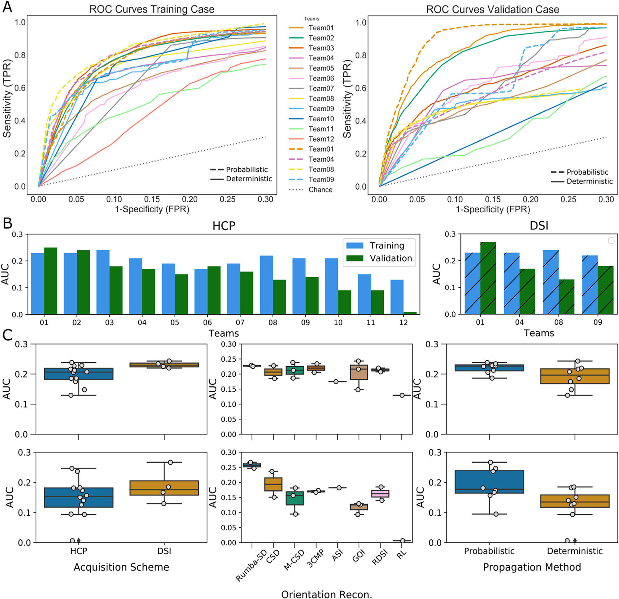
(A) ROC curves are shown for each submission. Results are shown for the training case (left) and validation case (right), and for the HCP (solid lines) and DSI (dashed line) acquisition schemes. (B) Bar plots show the AUC score for each submission for the training case (blue) and validation (green) case, and for HCP and DSI sampling schemes. (C) AUC scores are shown by acquisition scheme, orientation reconstruction method, and tractography propagation method for the training case (top) and the validation case (bottom). Rumba-SD = robust and unbiased model-based spherical deconvolution(Canales-Rodríguez et al., 2015); CSD= constrained spherical deconvolution (Tournier et al., 2007); M-CSD = multi-shell multi-tissue CSD (Dhollander et al., 2019; Jeurissen et al., 2014); 3Comp = three compartment model(Tran and Shi, 2015); ASI = asymmetry spectrum imaging (Wu et al., 2019); GQI = generalized Q-ball imaging (Yeh et al., 2010); RL= Richardson Lucy (Dell’Acqua et al., 2010), RDSI = radial diffusion spectrum imaging (Baete et al., 2019, 2016).

3.2. Sensitivity varies across white matter regions

We investigated how many of the white matter regions included in the tracer mask were correctly labeled by each Submission. Fig. 3 shows the TPR of each submission at the same specificity level (FPR=0.1) for different white matter ROIs labeled in the training and validation case (2.4.2 Bundle-wise TPR). Sensitivity was variable across regions, with similar patterns across submissions. In the training case, most teams labeled the EC, CC, and MPF correctly, but could reach the UF and CB only partially (Fig. 3A).

Fig. 3. Performance by white-matter region.

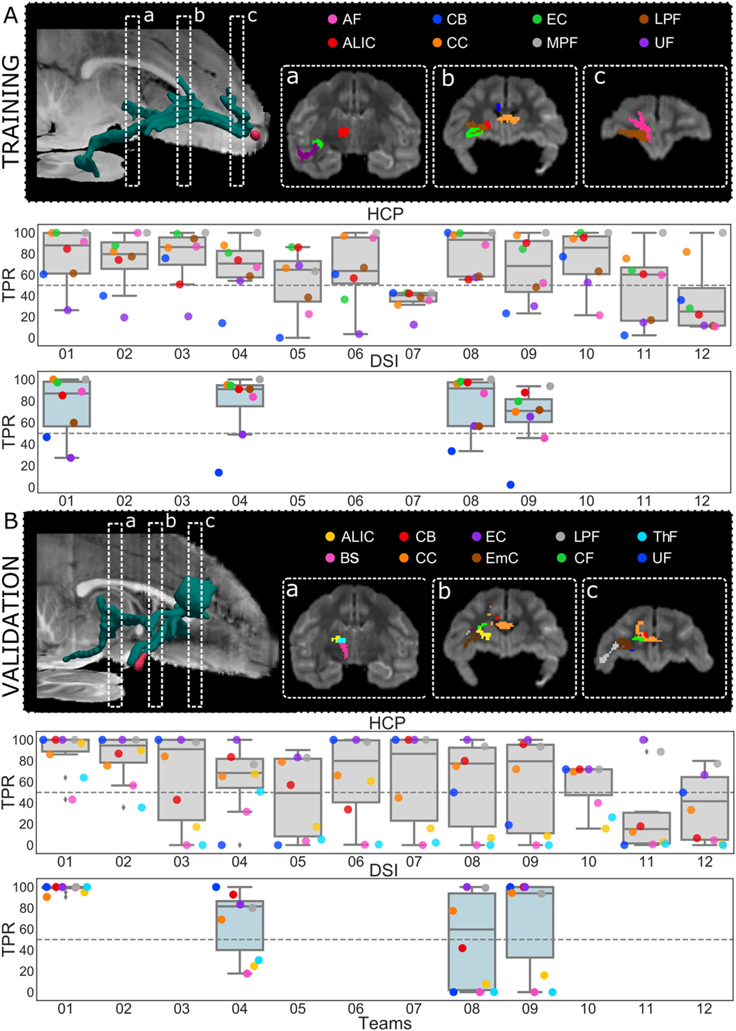
(A) 3D rendering of the tracer mask (in green) and injection site (in red) for the training case, showing the location of the coronal slices that are displayed in boxes a, b, and c. The boxes show the main white-matter pathways present in the tracing. Boxplots overlaid with scatterplots show the TPR in each bundle for each submission, with the HCP scheme (top, light grey) and the DSI scheme (bottom, light blue). (B) The same results are presented for the validation case. All TPRs were evaluated at FPR=0.1. (AF = anterior frontal white matter; ALIC=anterior limb of the internal capsule; BS= brainstem fibers; CB = cingulum bundle; CC = corpus callosum; CF = commissural fibers; EC = external capsule; EmC = extreme capsule; LPF = lateral pre-frontal white matter; MPF = medial pre-frontal white matter; OF = orbitofrontal white matter; ThF = thalamic fibers; UF = uncinate fasciculus).

In the validation case, almost all methods could label the UF, EC, and LPF correctly but most of the submissions failed to reach regions located at a greater distance from the injection site, like the BS, ThF, and ALIC. In the training case several teams achieved similar performance as Team 1. In the validation case, however, where fine-tuning with respect to the ground truth was not possible, the performance of most teams deteriorated. The best result was achieved by the Rumba-SD model (Canales-Rodríguez et al., 2015) and probabilistic tractography (Garyfallidis et al., 2014; Girard et al., 2014) on the DSI data (Team 1), which achieved a TPR higher than 0.9 for all the regions. There were clear differences in the bundles where errors occurred in the training vs. the validation case. This has to do with the fact that fibers starting from the two different injection sites enter these bundles from different angles (See 3.4 Branching and turning fiber configurations are challenging for tractography).

3.3. Round 2 results (standardized pre- and post-processing)

Fourteen teams completed round 2 (259 total submission. Training: 105. Validation: 154). Of these, eleven also completed round 1, one completed round 1 but submitted results with a different pipeline in round 2, and two teams were new (Team 13 and Team 14). Some of the teams that had completed round 1 submitted results with new methods, in addition to regenerating results with the methods that they had used in round 1 but with the standardized pre- and post-processing. Fifty final submissions were ranked (Supplementary Table 2).

Results show that the performance of most returning teams improved when compared to round 1, as a result of applying the harmonized pre- and post-processing strategies. This improvement was greater for the validation case (2–85%) than the training case (2–30%) (Fig. 4A). As a result, the difference in AUC score between the training and validation case decreased substantially in round 2 (Fig. 4B). This led to many more teams achieving more similar performance between the training and validation case (Supplementary Fig. 3). At the same FPR = 0.1, all submissions achieved higher TPR than in round 1 (Supplementary Fig. 4).

Fig. 4. Effect of harmonized pre- and post-processing.

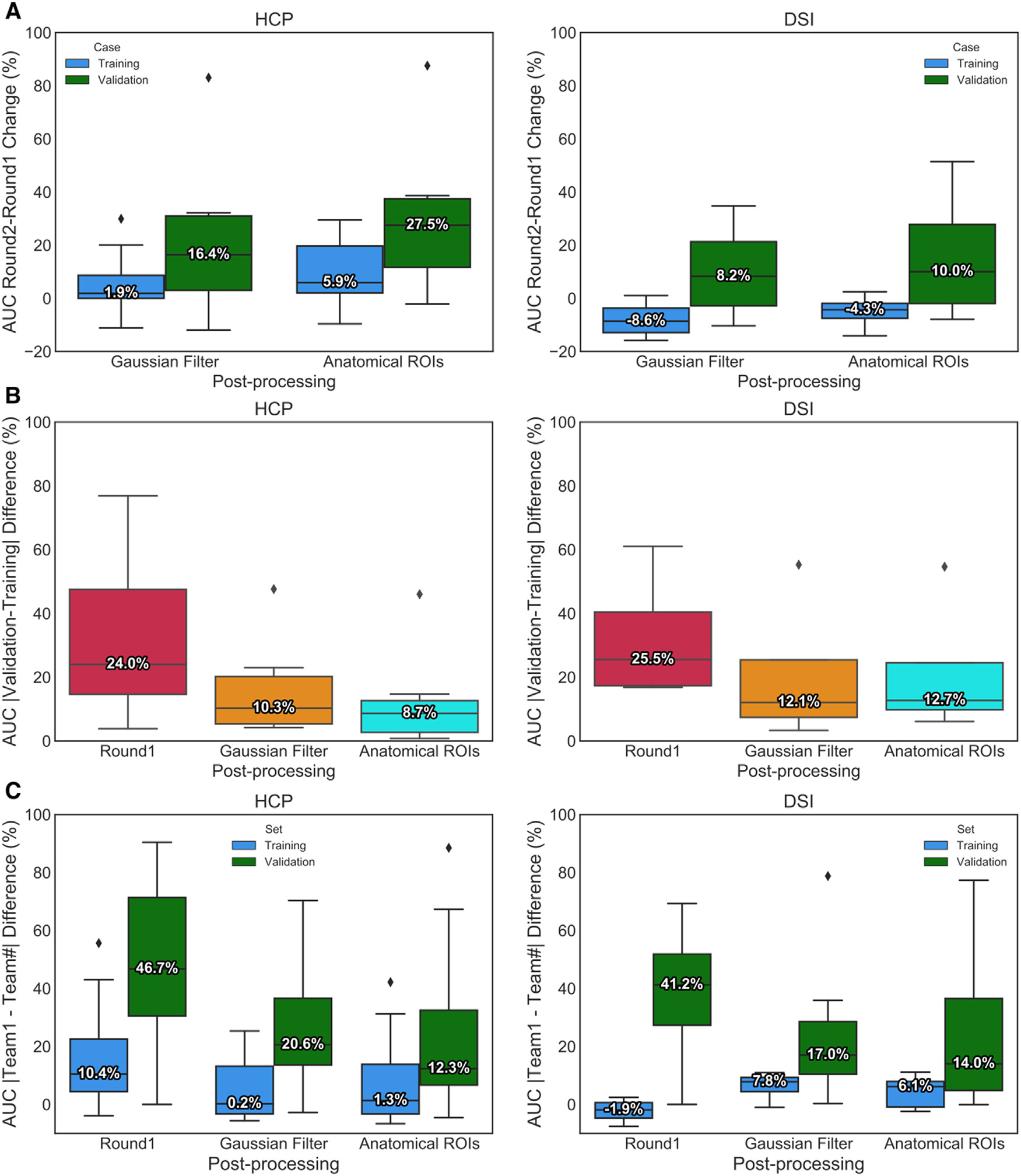
(A) Boxplots show the percent change in AUC scores between round 1 and round 2 for both post-processing strategies (Gaussian filter and anatomical ROIs). Results are shown for the training case (blue) and validation case (green), and for the HCP (left) and DSI (right) acquisition schemes. (B) Difference in AUC scores between the training and validation cases, for round 1 and for each of the two post-processing strategies in round 2 (Gaussian Filter and Anatomical ROIs). (C) We show the difference between the AUC score achieved in round 1 by Team 1 and the AUC scores achieved by all other submissions in round 1 and the two post-processing strategies in round 2. Median percent change is indicated by a horizontal line in each plot.

Remarkably, post-processing by Gaussian filtering, which does not assume any prior anatomical knowledge, also improved results for most submissions (Fig. 4B), leading to a training-validation percent difference only slightly higher than the one obtained when using the anatomical ROIs. Only two teams (Team 6 and Team 8) did not show improvement with Gaussian filtering and one of them (Team 8) did not show improvement with anatomical ROIs. These improvements allowed most teams to obtain higher scores, reducing the difference between their performance and that of Team 1, especially for the validation case (Fig. 4C).

Fig. 5 shows ROC curves for round 2 with the bundle-wise TPR, i.e., the portion of white-matter regions where each submission achieved at least 50% coverage. For this and subsequent results presented in this section, we show only one submission per team (the one that achieved the highest AUC score on the validation case). Results are shown for post-processing by a Gaussian filter. Some of the submissions that used deterministic tractography (Team 8 for HCP and DSI schemes; Team 12 for HCP scheme) could not reach all the ten white-matter regions and are thus not shown. There was considerable variability across submissions, with Teams 1 and 2 reaching 50% coverage of all the regions with FPR < 0.11, and the remaining submissions with FPR > 0.15. Deterministic methods (solid lines) operate at lower specificity levels, and are only able to reach all regions at the cost of FPR > 0.22. In some cases, submissions that used the same orientation reconstruction method (M-CSD (Dhollander et al., 2019; Jeurissen et al., 2014)) achieved coverage of all regions at very different FPR levels, suggesting that other algorithmic choices had an impact on the TPR/FPR trade-off. It is worth noting that for the DSI scheme, all submissions (including deterministic) reached all ten regions at higher specificity levels (FPR ≤ 0.15) than for the HCP scheme, and that the submission that used Rumba-SD was able to reach 9 out of 10 regions with an FPR as low as 0.06.

Fig. 5. Bundle-wise TPR.

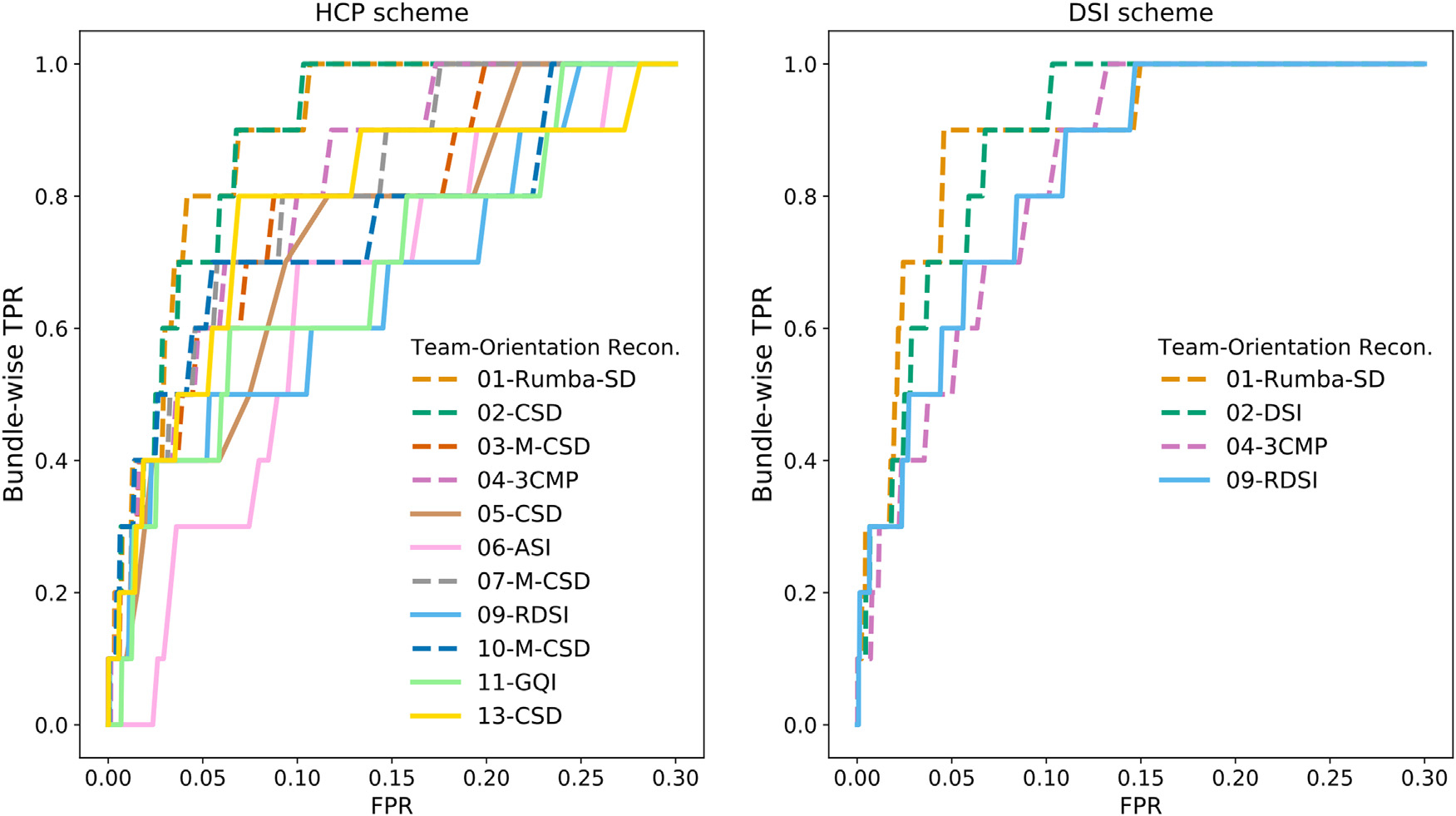
ROC curves with the bundle-wise TPR are shown for the validation case and post-processing by a Gaussian filter. The bundle-wise TPR is defined as the portion of white-matter regions (ALIC, BS, CB, CC, CF, EC, EmC, LPF, ThF, UF) where a submission achieved at least 50% coverage. ASI = asymmetry spectrum imaging(Wu et al., 2018); 3CMP = three compartment model (Tran and Shi, 2015); CSD = constrained spherical deconvolution (Tournier et al., 2007); DSI = Diffusion spectrum imaging (Wedeen et al., 2005); GQI = generalized Q-ball imaging (Yeh et al., 2010); M-CSD = multi-shell multi-tissue CSD (Dhollander et al., 2019; Jeurissen et al., 2014); RDSI = radial diffusion spectrum imaging (Baete et al., 2019, 2016); Rumba-SD = robust and unbiased model-based spherical deconvolution (Canales-Rodríguez et al., 2015).

Fig. 6 shows the tractogram threshold for which each team achieved bundle-wise TPR = 0.8. Overall, most submissions needed very relaxed thresholds (< 0.02 of the maximum value in the tractogram). Only one submission, using ASI (Wu et al., 2019) and deterministic tractography (Wu et al., 2020), achieved this coverage at a much more stringent threshold (0.13 of the maximum value in the tractogram). However, this submission also produced a much higher FPR at that threshold. For most submissions, a slightly higher (more stringent) threshold was needed in the validation case than the training case.

Fig. 6. Tractogram thresholds needed to achieve high coverage of the tracer mask.

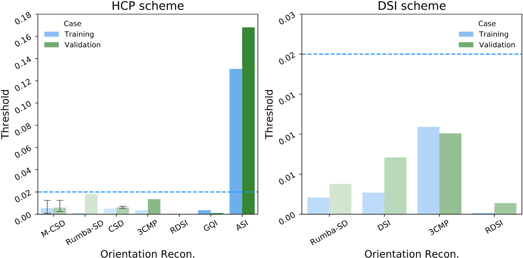
Bar plots show the tractogram threshold (with respect to the maximum value in the tractogram) for which each submission achieved bundle-wise TPR = 0.8. Submissions are grouped by the orientation reconstruction method that they used. Results are shown for the training (blue) and validation (green) case, and for the HCP (left) and DSI (right) sampling scheme. The bars are ordered along the x-axis by the FPR of the corresponding submissions, which is also indicated by the saturation level of each bar. ASI = asymmetry spectrum imaging (Wu et al., 2019, 2018); 3CMP = three compartment model (Tran and Shi, 2015); CSD = constrained spherical deconvolution (Tournier et al., 2007); DSI = Diffusion spectrum imaging (Wedeen et al., 2005); GQI = generalized Q-ball imaging (Yeh et al., 2010); M-CSD = multi-shell multi-tissue CSD (Dhollander et al., 2019; Jeurissen et al., 2014); RDSI = radial diffusion spectrum imaging (Baete et al., 2019, 2016); Rumba-SD = robust and unbiased model-based spherical deconvolution (Canales-Rodríguez et al., 2015).

Supplementary Fig. 5 shows the MHD between the tracer mask and the tractogram plotted against the TPR. While the FPR penalizes all FPs equally, the MHD measures how far from the tracer mask the FPs occur. The plots show that the MHD was greater for the validation than the training case for all submissions, even those that achieved similarly high AUC score in the two cases. At the same sensitivity level, MHD was greater for deterministic than probabilistic methods. Similarly to what we observed with the bundle-wise ROCs of Fig. 5, there were submissions that used the same orientation reconstruction method (CSD) but had very different MHDs at the same level of sensitivity (3–8 mm range at TPR = 0.8). The MHD was below 10 mm for all submissions and all levels of sensitivity.

3.4. Branching and turning fiber configurations are challenging for tractography

Fig. 7 shows histograms of the number of teams that achieved a TP (i.e., voxels included both in the tractogram and in the tracer mask) in each voxel of the tracer mask, at FPR = 0.1.

Fig. 7. Number of teams reaching each voxel in the tracer mask.

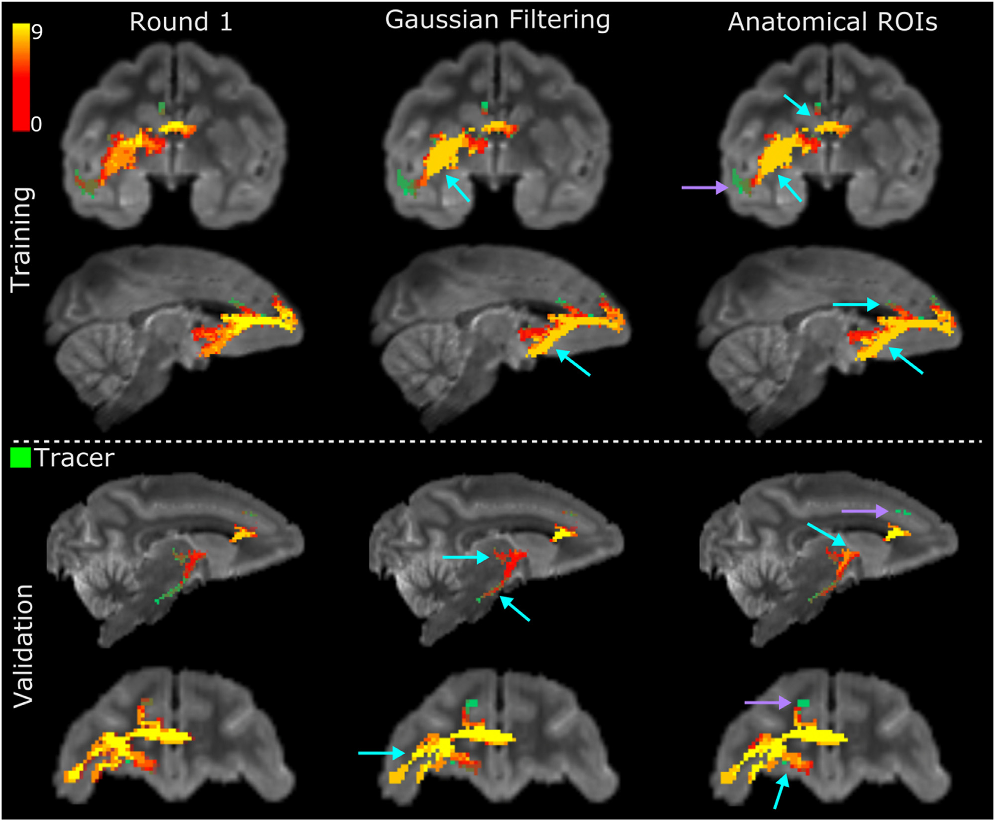
The heat maps are maximum intensity projections of the histograms of TPs across teams at FPR = 0.1, for the HCP acquisition scheme. The tracer mask is shown in green, under the heat maps. Results are shown for the training and validation case, and for round 1 and the two filtering strategies (Gaussian filtering, anatomical ROIs) in round 2. Only submissions that completed both rounds were included. Cyan arrows point to regions where the standardized pre- and post-processing round 2 led to improvement with respect to round 1. Violet arrows point to regions that remained challenging in both rounds.

These histograms are shown for round 1 and for each of the post-processing strategies adopted in round 2. The pre- and post-processing used in round 2 improved the overall coverage of the tracer masks by tractography. In the training case, the ALIC, CB, EC were labeled correctly by most teams (Fig. 7, top, light blue arrows), while only few teams could label these regions in round 1. The region where fibers turn sharply towards the temporal terminations of the UF remained challenging for all teams in both rounds (Fig. 7, top, violet arrow). In the validation case, the biggest improvement was located where fibers coming from the ALIC branch into fibers entering the thalamus and fibers entering a narrow bundle of axons projecting down the brainstem. In round 2, more submissions labeled the thalamic fibers correctly and achieved improved coverage of the inferior brainstem fibers. Despite this improvement, this region continues to pose challenges for most teams (Fig. 7, bottom, violet arrow). Like the UF region, this branch point is located further away from the injection/seed point than other regions in the tracing mask. Therefore, tractography needs to traverse other branching and turning points to get there and, as errors accumulate, the number of streamlines that reach these regions is small.

We can better understand the nature of these errors by examining the false positives that occur around these challenging areas. We identified two regions for the training case (UF and LPF) and two for the validation case (ALIC and EC) where the tracer and tractography trajectories consistently diverged in most submissions (Fig. 8, Supplementary video). We observed that in areas where fibers branch into two bundles, tractography tends to follow the least curved of the two and miss the other. Similarly, in areas where fibers take a sharp turn but, at the resolution of the dMRI data, overlap with a separate, less curved pathway, tractography follows the latter, instead of taking the turn. An example of such configuration is the area where the fibers coming from the EC turn towards the UF and the ILF (Fig. 8B). Here tractography follows the ILF erroneously and fails to reach the UF terminations in the temporal lobe.

Fig. 8. Challenging areas for tractography.

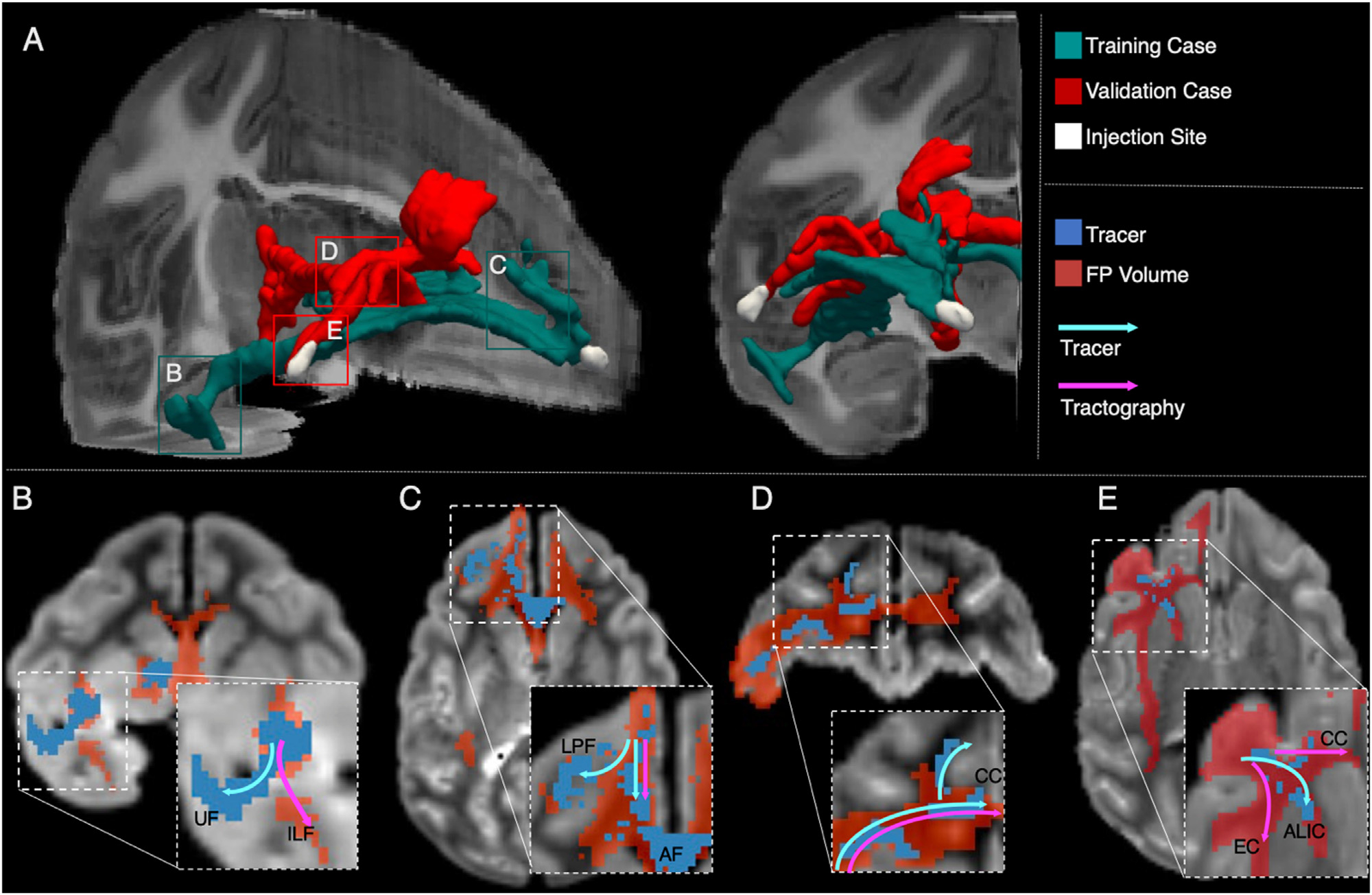
(A) 3D rendering of the tracer and injection site for the training (green) and validation (red) cases. Labeled boxes show the location of 2D views presented in B-E. (B, C) A map of FPs is shown for one representative submission at FPR = 0.1 (red), overlaid by the tracer mask (blue) for the training case. Streamlines follow the ILF, instead of turning into the UF (B). Streamlines continue into the AF instead of fanning into the LPF (C). (D, E) A map of FPs is shown for one representative submission at FPR = 0.1 (red), overlaid by the tracer mask (blue) for the validation case. Streamlines continue in the body of the CC to project contralaterally and miss the turn into the superior frontal gyrus (D). Tractography follows paths of lower curvature in the body of the CC and in the EC, instead of projecting into the ALIC (E). AF: antero-frontal white matter; ALIC: anterior limb of the internal capsule; CC: corpus callosum; EC: external capsule; ILF: inferior longitudinal fasciculus; LPF: lateral pre-frontal white matter; UF: uncinate fasciculus.

Fanning regions also lead to errors in tractography. In the training case, fibers exiting the injection site branch from the main bundle, which is sometimes referred to as the “stalk”, and fan out towards the dorsolateral prefrontal cortex. Here tractography follows the main stalk, continuing in the frontal white matter and does not turn superolateral to then fan into the LPF (Fig. 8C). In the validation case, most teams showed false negatives in the supero-frontal projections of the CC (Fig. 7). Fig. 8D shows that here tractography continues into the body of the CC to project to contralateral areas, missing the sharp turn of CC projections to the superior frontal gyrus. Another region of the validation case that showed significant false negatives across submissions was the region where fibers enter the ALIC. Here tractography prefers following the direction of least curvature in the CC body and into the big bundle of anterior-posterior fibers stemming from the EC, rather than turning into the smaller ALIC (Fig. 8E).

3.5. Sharper diffusion profiles do not always lead to more accurate tractography

We compared the ODFs from different submissions in an area that was consistently challenging across methods. This was where fibers branched into thalamic and brainstem fibers (Fig. 7). All submissions identified two fiber populations correctly in the superior part of this region, where fibers branched, and one main fiber population in the inferior part, where fibers projected caudally to the brainstem. However, there were differences in the sharpness of the ODFs. Interestingly, the submissions that achieved the highest accuracy were not the ones with the sharpest diffusion profiles. This suggests that, depending on the underlying fiber configuration, ODF sharpness may not be a universally desirable property. Especially in the superior part of the ROI, where the two sets of fibers diverge, the best performing teams (Fig. 9B–D) show somewhat less sharp ODFs. However, no clear trend was visible across submissions as some of the submissions achieving lower accuracy also show less sharp ODFs.

Fig. 9. Comparison of ODFs across submissions.

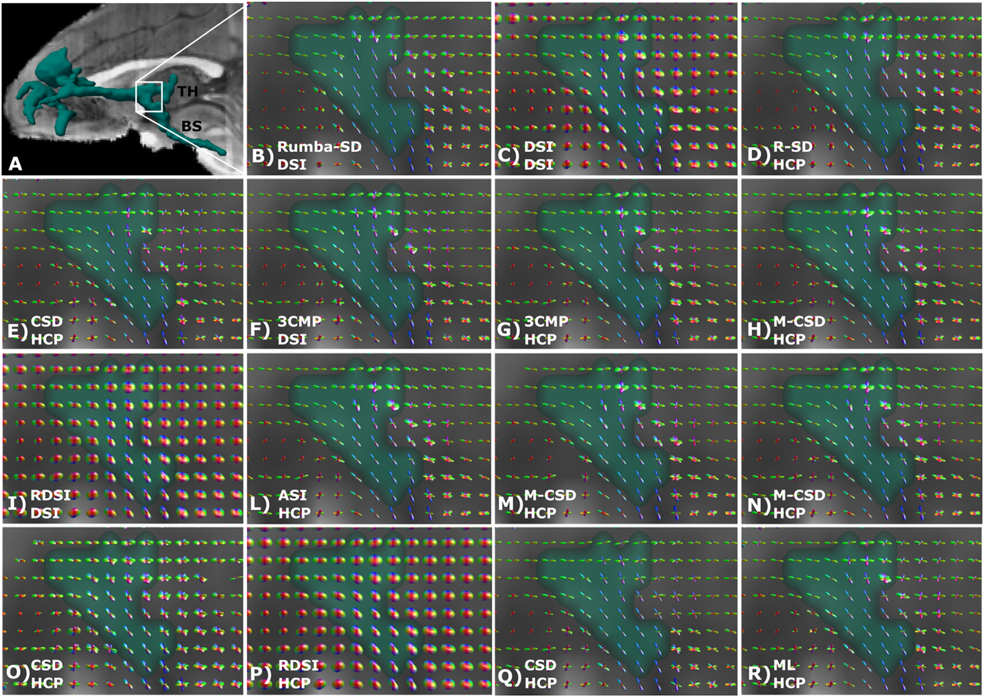
(A) 3D rendering of the tracer mask from the validation case, showing the location of the magnification region where thalamic (TH) and brainstem (BS) fibers branch. (B–R) ODFs for each submission are visualized for the region shown in A. Submissions are ordered based on the AUC score obtained for the validation case in round 2. ASI: asymmetry spectrum imaging (Wu et al., 2019); 3CMP: three compartment model (Tran and Shi, 2015); CSD: constrained spherical deconvolution (Tournier et al., 2007); DSI: Diffusion spectrum imaging (Wedeen et al., 2005); M-CSD: multi-shell multi-tissue CSD (Dhollander et al., 2019; Jeurissen et al., 2014); ML: machine learning-based reconstruction (Karimi et al., 2021); RDSI: radial diffusion spectrum imaging (Baete et al., 2019, 2016); Rumba-SD: robust and unbiased model-based spherical deconvolution (Canales-Rodríguez et al., 2015).

We quantified the sharpness of the ODFs by computing the dispersion of each peak in each voxel. Fig. 10 shows plots of the average dispersion in seven ROIs from the training and validation case. We selected both regions with complex fiber configurations (UF, CB, CC, EC-IC, TH-BS) and regions that should mainly contain single fiber orientations, like the body of the CC (CCb) and BS. Fig. 10 shows that, although ODF dispersion was not the only factor that determined accuracy, submissions that achieved higher AUC scores had less sharp ODFs, especially in regions with turning, fanning, and branching fiber configurations (TH-BS, CC, UF). This variability across regions was confirmed by correlating the AUC with the mean dispersion across all ROIs from the training and validation cases. Results show a lack of such a correlation for both HCP and DSI data (Supplementary Fig. 6).

Fig. 10. Effect of ODF dispersion and peak orientation on the accuracy of tractography.

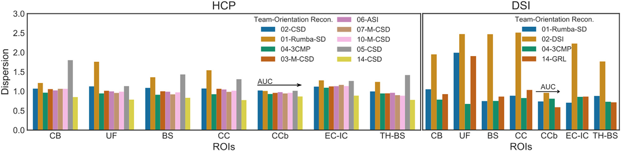
Bar plots of mean dispersion for each submission and each sampling scheme across different ROIs from the training and validation cases. For each ROI, teams are ordered along the x-axis based on AUC score for the validation case in round 2. Note that, as dispersion affects only methods that sample orientations from ODF, we excluded methods that follow the peak orientation exclusively. Training case: CB = cingulum bundle, UF = uncinate fasciculus. Validation case: BS = brainstem, CC = corpus callosum, CCb = body of the corpus callosum, EC-IC = external capsule – internal capsule, TH-BS = thalamus – brainstem. ASI = asymmetry spectrum imaging (Wu et al., 2019); 3CMP = three compartment model (Tran and Shi, 2015); CSD = constrained spherical deconvolution (Tournier et al., 2007); DSI = Diffusion spectrum imaging (Wedeen et al., 2005);; M-CSD = multi-shell multi-tissue CSD (Dhollander et al., 2019); GRL= generalized Richardson-Lucy (Guo et al., 2019); ML = machine learning-based reconstruction (Karimi et al., 2021); RDSI = radial diffusion spectrum imaging (Baete et al., 2019, 2016); Rumba-SD = robust and unbiased model-based spherical deconvolution (Canales-Rodríguez et al., 2015).

4. Discussion

The IronTract Challenge evaluated a variety of state-of-the-art tractography methods on high-angular and spatial resolution dMRI data by quantitative voxel-wise comparison to anatomic tracing data in the same NHP brains. This effort differed from previous tractography challenges in several ways. First, the dMRI acquisition protocol allowed us to evaluate HCP-style and DSI acquisition schemes in real brain data. Second, the availability of both dMRI and tracer data in the same brains allowed the precise localization of tractography errors and challenging fiber configurations. Third, a training and validation case with different injection sites allowed us to evaluate the robustness of submissions across seed areas. Fourth, a full ROC analysis allowed us to compare the sensitivity of different methods at the same level of specificity. Fifth, by iterating over the results in a second round, where all teams used the same pre- and post-processing steps, we disentangled the contribution of these steps from that of the orientation reconstruction and tractography steps. Our results provide insights into the optimal processing strategies for widely available, HCP-style data. They also reveal why errors occur even with these state-of-the-art acquisition and analysis techniques, thus pointing to possible areas of improvement for future methodological development.

4.1. The effect of acquisition scheme and propagation method

We compared an HCP-style, two-shell acquisition scheme with a much more densely sampled DSI scheme. Overall, higher accuracy was achieved by methods that used the full DSI data (515 diffusion volumes) (Fig. 2). However, a few of the methods that used the HCP data approached the accuracy of the DSI methods. For methods that could be applied to both schemes, the loss in accuracy when using HCP versus DSI data was lower than 10% (Supplementary Table 1, Fig. 2). This illustrates that when analysis methods are carefully optimized, the two-shell HCP scheme represents an advantageous trade-off between accuracy and acquisition time, given that DSI acquisition involves 2.8 times more directions and 3.3 times higher maximum b-value. Previous validation studies showed that DSI produces more accurate fiber orientation estimates both in simulations (Daducci et al., 2014) and in comparison to optical imaging measurements (Jones et al., 2020). In this study, the most accurate submission was obtained using DSI data. While a full DSI acquisition is time-consuming, compressed sensing (CS) allows DSI data to be reconstructed from undersampled q-space (Menzel et al., 2011; Setsompop et al., 2013; Tobisch et al., 2018). A recent post mortem validation study showed that a CS-DSI protocol with 171 directions (similar to the number of directions in the two-shell HCP protocol), preserves the high angular accuracy of fully sampled DSI (Jones et al., 2021). Thus, it is a viable alternative that combines the benefits of shell and grid acquisitions.

In regard to the propagation method, we found that probabilistic tractography led to overall higher AUC (mean AUC: 0.22) than deterministic tractography (mean AUC = 0.17). This was particularly true for the validation case, where pipelines were not optimized with respect to the ground truth (Fig. 2A and C). This confirms the overall lower sensitivity of deterministic approaches at the same level of specificity (Girard et al., 2020; Grisot et al., 2021). Probabilistic tractography led to better bundle coverage (Fig. 5). Three deterministic submissions could not reach all the bundles labeled in the validation case, and the other ones did so at a much higher FPR than the probabilistic methods (Fig. 5). This was especially true for white matter regions located further away from the injection site/seed (Fig. 3B).

4.2. The effect of orientation reconstruction method

Differences between the ODFs from the various submissions were mostly subtle. Our results suggest that there is no simple, one-to-one mapping between ODF characteristics and the accuracy of tractography (Fig. 10, Supplementary Fig. 6). This result is in line with a recent study that found that there is no single optimal method for all different fiber configurations (Canales-Rodríguez et al., 2019).

However, the dispersion of the ODFs does seem to play a role. The conventional wisdom is that sharper ODFs are better because they help resolve crossing fibers with small inter-fiber angles (Canales-Rodríguez et al., 2019). However, the ODFs from the winning method (Rumba-SD) showed higher dispersion than ODFs from most of the other submissions. This was the case in almost all selected ROIs and especially in those that included branching, fanning, or turning fibers (Fig. 10). Less sharp ODFs, when combined with probabilistic tractography, allow a broader range of orientations to be sampled from the same ODF peak. This can be beneficial in areas of branching or fanning. Areas where fibers take sharp turns remain a challenge for all methods. They can only be resolved by relaxing bending angle thresholds to a degree where the FPR becomes prohibitively high.

In a previous study, we evaluated a different set of tractography methods on the dataset that we refer to as the training set here (Grisot et al., 2021). We observed the highest accuracy from the combination of probabilistic tractography with GQI, a reconstruction method that does not produce particularly sharp ODFs. The performance of probabilistic GQI in that study (TPR < 0.7 at FPR = 0.1) was lower than the performance of probabilistic Rumba-SD in the present study (TPR = 0.74 at FPR = 0.1). However, it may be worth revisiting the probabilistic GQI approach with the optimized pre- and post-processing methods of the IronTract Challenge.

4.3. The effect of pre- and post-processing

In the second round of the challenge, we investigated the extent to which the pre- and post-processing strategies had contributed to the higher robustness achieved by Teams 1 and 2 in the first round. When the remaining teams used the same strategies, accuracy improved for almost all submissions (Fig. 4). This improvement was higher for the validation than the training case, i.e., the accuracy of tractography became more robust to the location of the seed region. More specifically, accuracy improved in some regions that proved challenging in round 1 (Fig. 7).

While we did not study the effects of the pre- and post-processing separately, prior work studied the effects of some pre-processing steps on the accuracy of diffusion orientation estimates (Daducci et al., 2014). They found that denoising improved orientation accuracy up to 30–40%. Approximately half of the teams had applied denoising in round 1 and only four teams had performed eddy-current correction. These steps were included in the standardized pre-processing of round 2.

The improved accuracy obtained with the use of a priori anatomical ROIs was expected. The more surprising result was that post-processing with a simple Gaussian filter, which requires no prior anatomical information, increased the AUC by up to 80%, a benefit similar to the use of anatomical ROIs (Supplementary Fig. 2). While harmonizing pre- and post-processing in round 2 decreased the difference in AUC score between all the submissions and Team 1, the latter continued to achieve the highest accuracy. When using DSI data, Team 1 could reach a much higher TPR than all other submissions (TPR = 0.96 at FPR=0.1), suggesting that its pre- and post-processing strategies were not the only factors contributing to its high performance.

4.4. Localization of challenging areas

Having data from anatomic tracing and dMRI in the same monkey brain allowed us to identify the regions where tractography errors occurred consistently across submissions. These included regions where fibers branched into smaller bundles, or where they took a sharp turn to enter a bundle (Figs. 7 and 8, Supplementary video). These results agree with previous validation studies (Grisot et al., 2021; Schilling et al., 2019a) and illustrate the importance of anatomic tracing for identifying realistic failure modes of tractography that go beyond the simple crossing fiber configurations used in digital or physical phantoms. Almost all submissions were successful in identifying projections that ran through major crossing regions (Figs. 3 and 7). However, many methods had trouble following fibers that branched into smaller bundles or fanned off the main bundle (Figs. 7 and 8). These results highlight the need for further validation and development of tractography methods that go beyond the crossing-fiber paradigm.

4.5. Robustness across seed areas

Our training and validation cases allowed us to evaluate the robustness of tractography methods across different seed areas. The two injection sites, while projecting through similar white-matter pathways (Fig. 3), follow very different routes to reach these pathways and pose different challenges to tractography. In the training case, the injection site is in the frontal pole. From here, most fibers travel straight posteriorly to enter the internal and external capsule. The most challenging areas are where fibers fan out into the LPF or turn into the UF and CB (Figs. 7 and 8). In the validation case, the injection site is in the vlPFC. From here, fibers need to first course medially and take a more complicated and curved trajectory before entering the capsules. The ALIC shows lower TPs in the validation case than in the training case (Fig. 3), and the most challenging area is located posterior to the ALIC where fibers branch into thalamic and brainstem fibers (Fig. 7).

For most of the submissions, optimizing the methods with respect to accuracy for one seed/injection region did not guarantee optimal performance for another region, with a 25% average decrease in AUC score between the training and the validation case (Fig. 2). Only two teams could achieve high accuracy for both injection sites. One of these two teams used anatomical ROIs, based on general knowledge on the connections of the prefrontal cortex from previous tracer experiments (Lehman et al., 2011), illustrating the importance of such experiments for mapping the organizational rules of white matter projections. In future studies, we intend to investigate a wider variety of injection sites and evaluate whether these conclusions generalize to different brain areas.

4.6. Optimal data processing for the HCP protocol

One of the main goals of the IronTract challenge was to identify optimal processing strategies for the widely used, two-shell HCP acquisition scheme. Our results can inform various methodological choices that have to be made when analyzing such data, including pre-processing, orientation reconstruction, tractography, post-processing, and thresholding. When these choices were made as summarized below, tractography reconstructed 8 out of the 10 bundles present in the tracer mask with FPR = 0.05, and it reconstructed all 10 with FPR = 0.1 (Fig. 5).

Pre-processing:

The winning pipeline included denoising (Veraart et al., 2016), corrections for Gibbs ringing (Kellner et al., 2016), and motion/eddy-current distortions (Andersson et al., 2003; Andersson and Sotiropoulos, 2015), all sensible and widely used procedures.

Orientation reconstruction:

The method that achieved the highest performance was Rumba-SD (Figs. 3, 5 and Supplementary Figs. 5 and 7). Its estimation framework relies on Rician and noncentral Chi likelihood models, which accommodate realistic MRI noise, and a 3D total-variation spatial regularization term, which promotes continuity and smoothness along individual tracts by taking into account the spatial correlation among adjacent voxels (Canales-Rodríguez et al., 2015). While this is a relatively newer method, we note that high accuracy and robustness were also achieved by classical reconstruction methods like CSD (Tournier et al., 2007) (applied on the high-b shell only) and DSI (Wedeen et al., 2005). However, these results were specific to Team 2, who supplemented these methods with anatomical ROIs. The 3CMP (Tran and Shi, 2015) and M-CSD (Dhollander et al., 2019; Jeurissen et al., 2014) also achieved relatively higher accuracy and lower reconstruction error than other methods (Figs. 5 and 6).

Tractography:

Our results concur with previous studies that showed the higher sensitivity of probabilistic methods, when compared to their deterministic counterparts at the same specificity (Girard et al., 2020; Grisot et al., 2021; Schilling et al., 2018).

Post-processing:

Simple Gaussian post-filtering improved the accuracy of most tractography methods used in this challenge, as well as their robustness to the location of the seed region. The use of inclusion ROIs based on prior anatomical knowledge led to small additional gains in performance.

Thresholding:

Most methods required a rather low threshold (< 2% of the maximum value of the tractogram) to reach all the main bundles present in the tracer (Fig. 6). This is in agreement with a prior finding that the biggest changes in tractograms occur between thresholds of approximately 2 and 3%, above which the sensitivity of tractography decreases dramatically (Schilling et al., 2019a). We note that we focused on optimal thresholds for reconstructing all the bundles that the injection site projects to, which is a task that requires high sensitivity. In other tasks, such as constructing whole-brain connectivity matrices, high specificity may be more important. In that case, where low specificity would lead to a situation where most brain regions appear to be connected to each other, one may want to use more stringent thresholds and accept that only a subset of the true connections will be included.

It is important to note that the outcomes of this study are based on ex vivo dMRI data and therefore the processing strategies suggested here may be supplemented with additional steps, such corrections for Rician noise correction (Koay and Basser, 2006) or susceptibility-induced distortions (Andersson et al., 2003), when analyzing in vivo data.

4.7. Limitations

The main limitation of using tracer injections to validate dMRI tractography is that such studies cannot be performed in the human brain. Human and NHP brains differ in terms of both absolute and relative sizes of different gray and white-matter structures. However, similarities in position, cytoarchitectonics, connections, and behavior indicate that the overall organization of brain circuitry is relatively comparable (Petrides et al., 2012; Petrides and Pandya, 1984). In particular, the relative positions of different brain regions, as well as the obstacles the fibers encounter on their way from one area to another, are comparable. As a result, similar fiber geometries (crossing, branching, turning, fanning) exist in similar locations of the NHP and human brain. Thus, important insights can be gained from the performance of tractography methods in NHP brains.

The present study was limited to two injection/seed areas. Furthermore, we used binary tracer and tractography maps, i.e., we only compared the presence or absence of labeled axons and tractography streamlines at each voxel, rather than their density. Automated methods for segmenting and quantifying the tracer maps will be critical for extending these analyses in the future.

Other limitations of tracer validation studies include imperfect tracer uptake or imperfect alignment of histology and dMRI data. The injections used in this study passed rigorous quality assurance checks at Dr. Haber’s laboratory and had high-quality transport. Injections that showed evidence of contamination or weak labeling were not included in this study (Haber et al., 2006). The manual annotation of the axon bundles and their alignment to the dMRI volumes were also checked by Dr. Haber and refined at multiple stages.

Finally, it should be noted that macaque brains are fixed by in situ perfusion, which limits the degradation of the tissue caused by autolysis in human post mortem brains (D’Arceuil and de Crespigny, 2007). Nonetheless, diffusivity is reduced in all post-mortem specimens when compared to in vivo brains. Previous studies have demonstrated that, while fixation decreases diffusivity by 60–80% compared to in vivo, diffusion anisotropy along fiber orientations is largely preserved (D’Arceuil and de Crespigny, 2007; Dyrby et al., 2011; McNab et al., 2009). We accounted for the decrease in diffusivity by multiplying the b-values in the dMRI protocol by a factor of 4. Some parameters of orientation reconstruction methods may have to be adjusted differently for ex vivo and in vivo tissue, therefore we have not provided recommendations on the values of such parameters.

5. Conclusion

As part of the IronTract challenge we undertook a comprehensive, quantitative, voxel-wise assessment of tractography accuracy across different tractography pipelines, acquisition schemes, and seed areas. This allowed us to identify common failure modes of tractography for both commonly used and more recently developed tractography algorithms and to propose optimized strategies for analyzing dMRI data that have been acquired with high angular resolution techniques, including the popular two-shell acquisition scheme employed by the lifespan and disease HCP. The IronTract Challenge remains open (https://qmenta.com/irontract-challenge/) and we plan to expand its scope in future iterations. We hope that it can serve as a valuable validation tool for both users and developers of dMRI analysis methods.

Data availability

The authors declare that the data supporting the findings of this study are available on the QMENTA platform (https://qmenta.com/irontract-challenge/). The post-processing scripts used in Round2 are available at https://github.com/chiaramff/IronTract. Detailed information on how to reproduce the tractograms generated by the challenge teams, and links to code repositories are provided in supplementary note 1 and supplementary note 2 in the supplementary information.

References

- Aganj I, Lenglet C, Sapiro G, Yacoub E, Ugurbil K, Harel N, 2010. Reconstruction of the orientation distribution function in single- and multiple-shell q-ball imaging within constant solid angle. Magn. Reson. Med. 64, 554–566. doi: 10.1002/mrm.22365. [DOI] [PMC free article] [PubMed] [Google Scholar]
- Ambrosen KS, Eskildsen SF, Hinne M, Krug K, Lundell H, Schmidt MN, van Gerven MAJ, Mørup M, Dyrby TB, 2020. Validation of structural brain connectivity networks: the impact of scanning parameters. Neuroimage 204, 116207. doi: 10.1016/j.neuroimage.2019.116207. [DOI] [PubMed] [Google Scholar]
- Andersson JLR, Skare S, Ashburner J, 2003. How to correct susceptibility distortions in spin-echo echo-planar images: application to diffusion tensor imaging. Neuroimage 20, 870–888. doi: 10.1016/S1053-8119(03)00336-7. [DOI] [PubMed] [Google Scholar]
- Andersson JLR, Sotiropoulos SN, 2015. An integrated approach to correction for off-resonance effects and subject movement in diffusion MR imaging. Neuroimage doi: 10.1016/j.neuroimage.2015.10.019. [DOI] [PMC free article] [PubMed] [Google Scholar]
- Avants BB, Epstein CL, Grossman M, Gee JC, 2008. Symmetric diffeomorphic image registration with cross-correlation: evaluating automated labeling of elderly and neurodegenerative brain. Med. Image Anal. 12, 26–41. doi: 10.1016/j.media.2007.06.004. [DOI] [PMC free article] [PubMed] [Google Scholar]
- Azadbakht H, Parkes LM, Haroon HA, Augath M, Logothetis NK, De Crespigny A, D’Arceuil HE, Parker GJM, 2015. Validation of high-resolution tractography against in vivo tracing in the macaque visual cortex. Cereb. Cortex 25, 4299. doi: 10.1093/CERCOR/BHU326, New York, NY. [DOI] [PMC free article] [PubMed] [Google Scholar]
- Baete SH, Cloos MA, Lin YC, Placantonakis DG, Shepherd T, Boada FE, 2019. Fingerprinting orientation distribution functions in diffusion MRI detects smaller crossing angles. Neuroimage 198, 231–241. doi: 10.1016/j.neuroimage.2019.05.024. [DOI] [PMC free article] [PubMed] [Google Scholar]
- Baete SH, Yutzy S, Boada FE, 2016. Radial q-space sampling for DSI. Magn. Reson. Med. 76, 769–780. doi: 10.1002/mrm.25917. [DOI] [PMC free article] [PubMed] [Google Scholar]
- Bookheimer SY, Salat DH, Terpstra M, Ances BM, Barch DM, Buckner RL, Burgess GC, Curtiss SW, Diaz-Santos M, Elam JS, Fischl B, Greve DN, Hagy HA, Harms MP, Hatch OM, Hedden T, Hodge C, Japardi KC, Kuhn TP, Ly TK, Smith SM, Somerville LH, Uğurbil K, van der Kouwe A, Van Essen D, Woods RP, Yacoub E, 2019. The lifespan human connectome project in aging: an overview. Neuroimage 185, 335–348. doi: 10.1016/J.NEUROIMAGE.2018.10.009. [DOI] [PMC free article] [PubMed] [Google Scholar]
- Canales-Rodríguez EJ, Daducci A, Sotiropoulos SN, Caruyer E, Aja-Fernández S, Radua J, Mendizabal JMY, Iturria-Medina Y, Melie-García L, Alemán-Gómez Y, Thiran JP, Sarró S, Pomarol-Clotet E, Salvador R, 2015. Spherical deconvolution of multichannel diffusion MRI data with non-Gaussian noise models and spatial regularization. PLoS One 10, e0138910. doi: 10.1371/journal.pone.0138910. [DOI] [PMC free article] [PubMed] [Google Scholar]
- Canales-Rodríguez EJ, Legarreta JH, Pizzolato M, Rensonnet G, Girard G, Patino JR, Barakovic M, Romascano D, Alemán-Gómez Y, Radua J, Pomarol-Clotet E, Salvador R, Thiran JP, Daducci A, 2019. Sparse wars: a survey and comparative study of spherical deconvolution algorithms for diffusion MRI. Neuroimage 184, 140–160. doi: 10.1016/J.NEUROIMAGE.2018.08.071. [DOI] [PubMed] [Google Scholar]
- Canales-Rodríguez EJ, Melie-García L, Iturria-Medina Y, 2009. Mathematical description of q-space in spherical coordinates: exact q-ball imaging. Magn. Reson. Med. 61, 1350–1367. doi: 10.1002/MRM.21917. [DOI] [PubMed] [Google Scholar]
- Caruyer E, Lenglet C, Sapiro G, Deriche R, 2013. Design of multishell sampling schemes with uniform coverage in diffusion MRI. Magn. Reson. Med. 69, 1534–1540. doi: 10.1002/mrm.24736. [DOI] [PMC free article] [PubMed] [Google Scholar]
- Casey BJ, Cannonier T, Conley MI, Cohen AO, Barch DM, Heitzeg MM, Soules ME, Teslovich T, Dellarco DV, Garavan H, Orr CA, Wager TD, Banich MT, Speer NK, Sutherland MT, Riedel MC, Dick AS, Bjork JM, Thomas KM, Chaarani B, Mejia MH, Hagler DJ, Daniela Cornejo M, Sicat CS, Harms MP, Dosenbach NUF, Rosenberg M, Earl E, Bartsch H, Watts R, Polimeni JR, Kuperman JM, Fair DA, Dale AM, 2018. The adolescent brain cognitive development (ABCD) study: imaging acquisition across 21 sites. Dev. Cogn. Neurosci 32, 43–54. doi: 10.1016/J.DCN.2018.03.001. [DOI] [PMC free article] [PubMed] [Google Scholar]
- Christiaens D, Reisert M, Dhollander T, Sunaert S, Suetens P, Maes F, 2015. Global tractography of multi-shell diffusion-weighted imaging data using a multi-tissue model. Neuroimage 123, 89–101. doi: 10.1016/j.neuroimage.2015.08.008. [DOI] [PubMed] [Google Scholar]
- D’Arceuil H, de Crespigny A, 2007. The effects of brain tissue decomposition on diffusion tensor imaging and tractography. Neuroimage 36, 64–68. doi: 10.1016/J.NEUROIMAGE.2007.02.039. [DOI] [PMC free article] [PubMed] [Google Scholar]
- Daducci A, Canales-Rodriguez EJ, Descoteaux M, Garyfallidis E, Gur Y, Lin YC, Mani M, Merlet S, Paquette M, Ramirez-Manzanares A, Reisert M, Rodrigues PR, Sepehrband F, Caruyer E, Choupan J, Deriche R, Jacob M, Menegaz G, Prckovska V, Rivera M, Wiaux Y, Thiran JP, 2014. Quantitative comparison of reconstruction methods for intra-voxel fiber recovery from diffusion MRI. IEEE Trans. Med. Imaging 33, 384–399. doi: 10.1109/TMI.2013.2285500. [DOI] [PubMed] [Google Scholar]
- Dauguet J, Peled S, Berezovskii V, Delzescaux T, Warfield SK, Born R, Westin CF, 2007. Comparison of fiber tracts derived from in-vivo DTI tractography with 3D histological neural tract tracer reconstruction on a macaque brain. Neuroimage 37, 530–538. doi: 10.1016/J.NEUROIMAGE.2007.04.067. [DOI] [PubMed] [Google Scholar]
- Dell’Acqua F, Scifo P, Rizzo G, Catani M, Simmons A, Scotti G, Fazio F, 2010. A modified damped Richardson-Lucy algorithm to reduce isotropic background effects in spherical deconvolution. Neuroimage 49, 1446–1458. doi: 10.1016/j.neuroimage.2009.09.033. [DOI] [PubMed] [Google Scholar]
- Dhollander T, Mito R, Raffelt D, Connelly A, 2019. Improved white matter response function estimation for 3-tissue constrained spherical deconvolution. Proc. Intl. Soc. Mag. Reson. Med 27, 555. [Google Scholar]
- Donahue CJ, Sotiropoulos SN, Jbabdi S, Hernandez-Fernandez M, Behrens TE, Dyrby TB, Coalson T, Kennedy H, Knoblauch K, Van Essen DC, Glasser MF, 2016. Using diffusion tractography to predict cortical connection strength and distance: A quantitative comparison with tracers in the monkey. J. Neurosci. 36, 6758–6770. doi: 10.1523/JNEUROSCI.0493-16.2016. [DOI] [PMC free article] [PubMed] [Google Scholar]
- Dubuisson MP, Jain AK, Lansing E, B, A.B., 1994. A modified Hausdorff distance for object matching cor- 1 Introduction two point sets A and B can be combined in the follow- 2 distance between point sets research supported by a. In: Proceedings of the 12th International Conference on Pattern Recognit, pp. 566–568. [Google Scholar]
- Dyrby TB, Baaré WFC, Alexander DC, Jelsing J, Garde E, Søgaard LV, 2011. An ex vivo imaging pipeline for producing high-quality and high-resolution diffusion-weighted imaging datasets. Hum. Brain Mapp. 32, 544–563. doi: 10.1002/hbm.21043. [DOI] [PMC free article] [PubMed] [Google Scholar]
- Edlow BL, McNab JA, Witzel T, Kinney HC, 2016. The structural connectome of the human central homeostatic network. Brain Connect 6, 187–200. doi: 10.1089/brain.2015.0378. [DOI] [PMC free article] [PubMed] [Google Scholar]
- Fan Q, Nummenmaa A, Witzel T, Zanzonico R, Keil B, Cauley S, Polimeni JR, Tisdall D, Van Dijk KRA, Buckner RL, Wedeen VJ, Rosen BR, Wald LL, 2014. Investigating the capability to resolve complex white matter structures with high b-value diffusion magnetic resonance imaging on the MGH-USC Connectom scanner. Brain Connect 4, 718–726. doi: 10.1089/brain.2014.0305. [DOI] [PMC free article] [PubMed] [Google Scholar]
- Feng L, Jeon T, Yu Q, Ouyang M, Peng Q, Mishra V, Pletikos M, Sestan N, Miller MI, Mori S, Hsiao S, Liu S, Huang H, 2017. Population-averaged macaque brain atlas with high-resolution ex vivo DTI integrated into in vivo space. Brain Struct. Funct. 222, 4131–4147. doi: 10.1007/s00429-017-1463-6. [DOI] [PMC free article] [PubMed] [Google Scholar]
- Fessler JA, Sutton BP, 2003. Nonuniform fast Fourier transforms using min-max interpolation. IEEE Trans. Signal Process. 51, 560–574. doi: 10.1109/TSP.2002.807005. [DOI] [Google Scholar]
- Gao Y, Choe AS, Stepniewska I, Li X, Avison MJ, Anderson AW, 2013. Validation of DTI Tractography-based measures of primary motor area connectivity in the squirrel monkey brain. PLoS One 8, 75065. doi: 10.1371/JOURNAL.PONE.0075065. [DOI] [PMC free article] [PubMed] [Google Scholar]
- Garyfallidis E, Brett M, Amirbekian B, Rokem A, van der Walt S, Descoteaux M, Nimmo-Smith I, Dipy Contributors D, 2014. Dipy, a library for the analysis of diffusion MRI data. Front. Neuroinform. 8, 8. doi: 10.3389/fninf.2014.00008. [DOI] [PMC free article] [PubMed] [Google Scholar]
- Girard G, Caminiti R, Battaglia-Mayer A, St-Onge E, Ambrosen KS, Eskildsen SF, Krug K, Dyrby TB, Descoteaux M, Thiran JP, Innocenti GM, 2020. On the cortical connectivity in the macaque brain: a comparison of diffusion tractography and histological tracing data. Neuroimage 221. doi: 10.1016/j.neuroimage.2020.117201. [DOI] [PubMed] [Google Scholar]
- Girard G, Whittingstall K, Deriche R, Descoteaux M, 2014. Towards quantitative connectivity analysis : reducing tractography biases. Neuroimage 98, 266–278. doi: 10.1016/j.neuroimage.2014.04.074. [DOI] [PubMed] [Google Scholar]
- Grisot G, Haber SN, Yendiki A, 2021. Diffusion MRI and anatomic tracing in the same brain reveal common failure modes of tractography. Neuroimage 239, 118300. doi: 10.1016/j.neuroimage.2021.118300. [DOI] [PMC free article] [PubMed] [Google Scholar]
- Guo F, Leemans A, Viergever MA, Dell’Acqua F, De Luca A, 2019. Generalized Richardson-Lucy (GRL) for analyzing multi-shell diffusion MRI data. Neuroimage 218. doi: 10.1016/j.neuroimage.2020.116948. [DOI] [PubMed] [Google Scholar]
- Haber S, 1988. Tracing intrinsic fiber connections in postmortem human brain with WGA-HRP. J. Neurosci. Methods 23, 15–22. doi: 10.1016/0165-0270(88)90017-9. [DOI] [PubMed] [Google Scholar]
- Haber SN, Fudge JL, McFarland NR, 2000. Striatonigrostriatal pathways in primates form an ascending spiral from the shell to the dorsolateral striatum. J. Neurosci. 20, 2369–2382. doi: 10.1523/jneurosci.20-06-02369.2000. [DOI] [PMC free article] [PubMed] [Google Scholar]
- Haber SN, Kim KS, Mailly P, Calzavara R, 2006. Reward-related cortical inputs define a large striatal region in primates that interface with associative cortical connections, providing a substrate for incentive-based learning. J. Neurosci. 26, 8368–8376. doi: 10.1523/JNEUROSCI.0271-06.2006. [DOI] [PMC free article] [PubMed] [Google Scholar]
- Hagmann P, Cammoun L, Gigandet X, Meuli R, Honey CJ, Wedeen VJ, Sporns O, 2008. Mapping the structural core of human cerebral cortex. PLoS Biol. 6, e159. doi: 10.1371/journal.pbio.0060159. [DOI] [PMC free article] [PubMed] [Google Scholar]
- Harms MP, Somerville LH, Ances BM, Andersson J, Barch DM, Bastiani M, Bookheimer SY, Brown TB, Buckner RL, Burgess GC, Coalson TS, Chappell MA, Dapretto M, Douaud G, Fischl B, Glasser MF, Greve DN, Hodge C, Jamison KW, Jbabdi S, Kandala S, Li X, Mair RW, Mangia S, Marcus D, Mascali D, Moeller S, Nichols TE, Robinson EC, Salat DH, Smith SM, Sotiropoulos SN, Terpstra M, Thomas KM, Tisdall MD, Ugurbil K, van der Kouwe A, Woods RP, Zöllei L, Van Essen DC, Yacoub E, 2018. Extending the human connectome project across ages: imaging protocols for the lifespan development and aging projects. Neuroimage 183, 972–984. doi: 10.1016/J.NEUROIMAGE.2018.09.060. [DOI] [PMC free article] [PubMed] [Google Scholar]
- Haynes WIA, Haber SN, 2013. The organization of prefrontal-subthalamic inputs in primates provides an anatomical substrate for both functional specificity and integration: Implications for basal ganglia models and deep brain stimulation. J. Neurosci. 33, 4804–4814. doi: 10.1523/JNEUROSCI.4674-12.2013. [DOI] [PMC free article] [PubMed] [Google Scholar]
- Jbabdi S, Sotiropoulos SN, Savio AM, Graña M, Behrens TEJ, 2012. Model-based analysis of multishell diffusion MR data for tractography: how to get over fitting problems. Magn. Reson. Med. 68, 1846–1855. doi: 10.1002/MRM.24204. [DOI] [PMC free article] [PubMed] [Google Scholar]
- Jeurissen B, Leemans A, Tournier JD, Jones DK, Sijbers J, 2013. Investigating the prevalence of complex fiber configurations in white matter tissue with diffusion magnetic resonance imaging. Hum. Brain Mapp. 34, 2747–2766. doi: 10.1002/hbm.22099. [DOI] [PMC free article] [PubMed] [Google Scholar]
- Jeurissen B, Tournier JD, Dhollander T, Connelly A, Sijbers J, 2014. Multi-tissue constrained spherical deconvolution for improved analysis of multi-shell diffusion MRI data. Neuroimage 103, 411–426. doi: 10.1016/j.neuroimage.2014.07.061. [DOI] [PubMed] [Google Scholar]
- Jones DK, 2003. Determining and visualizing uncertainty in estimates of fiber orientation from diffusion tensor MRI. Magn. Reson. Med. 49, 7–12. doi: 10.1002/mrm.10331. [DOI] [PubMed] [Google Scholar]
- Jones DK, Alexander DC, Bowtell R, Cercignani M, Dell’Acqua F, McHugh DJ, Miller KL, Palombo M, Parker GJM, Rudrapatna US, Tax CMW, 2018. Microstructural imaging of the human brain with a ‘super-scanner’: 10 key advantages of ultra-strong gradients for diffusion MRI. Neuroimage doi: 10.1016/j.neuroimage.2018.05.047. [DOI] [PubMed] [Google Scholar]
- Jones DK, Knösche TR, Turner R, 2013. White matter integrity, fiber count, and other fallacies: the do’s and don’ts of diffusion MRI. Neuroimage 73, 239–254. doi: 10.1016/j.neuroimage.2012.06.081. [DOI] [PubMed] [Google Scholar]
- Jones R, Grisot G, Augustinack J, Magnain C, Boas DA, Fischl B, Wang H, Yendiki A, 2020. Insight into the fundamental trade-offs of diffusion MRI from polarization-sensitive optical coherence tomography in ex vivo human brain. Neuroimage 214, 116704. doi: 10.1016/j.neuroimage.2020.116704. [DOI] [PMC free article] [PubMed] [Google Scholar]
- Jones R, Maffei C, Augustinack J, et al. , 2021. High-fidelity approximation of grid- and shell-based sampling schemes from undersampled DSI using compressed sensing: Post mortem validation. Neuroimage 244, 118621. doi: 10.1016/j.neuroimage.2021.118621. [DOI] [PMC free article] [PubMed] [Google Scholar]
- Karimi D, Vasung L, Jaimes C, Machado-Rivas F, Khan S, Warfield SK, Gholipour A, 2021. A machine learning-based method for estimating the number and orientations of major fascicles in diffusion-weighted magnetic resonance imaging. Med. Image Anal. 72. doi: 10.1016/j.media.2021.102129. [DOI] [PMC free article] [PubMed] [Google Scholar]
- Kellner E, Dhital B, Kiselev VG, Reisert M, 2016. Gibbs-ringing artifact removal based on local subvoxel-shifts. Magn. Reson. Med. 76, 1574–1581. doi: 10.1002/mrm.26054. [DOI] [PubMed] [Google Scholar]
- Kremer JR, Mastronarde DN, McIntosh JR, 1996. Computer visualization of three-dimensional image data using IMOD. J. Struct. Biol. 116, 71–76. doi: 10.1006/jsbi.1996.0013. [DOI] [PubMed] [Google Scholar]
- Lehman JF, Greenberg BD, McIntyre CC, Rasmussen SA, Haber SN, 2011. Rules ventral prefrontal cortical axons use to reach their targets: implications for diffusion tensor imaging tractography and deep brain stimulation for psychiatric illness. J. Neurosci. 31, 10392–10402. doi: 10.1523/JNEUROSCI.0595-11.2011. [DOI] [PMC free article] [PubMed] [Google Scholar]
- Maffei C, Girard G, Schilling KG, Adluru N, Aydogan DB, Hamamci A, Yeh FC, Mancini M, Wu Y, Sarica A, Teillac A, Baete SH, Karimi D, Lin YC, Boada F, Richard N, Hiba B, Quattrone A, Hong Y, Shen D, Yap PT, Boshkovski T, Campbell JSW, Stikov N, Pike GB, Bendlin BB, Prabhakaran V, Alexander AL, Anderson A, Landman BA, Canales-Rodríguez EJ, Barakovic M, Rafael-Patino J, Yu T, Rensonnet G, Schiavi S, Daducci A, Pizzolato M, Fischi-Gomez E, Thiran JP, Dai G, Grisot G, Lazovski N, Puente A, Rowe M, Sanchez I, Prchkovska V, Jones R, Lehman J, Haber S, Yendiki A, 2020. The IronTract challenge: validation and optimal tractography methods for the HCP diffusion acquisition scheme. In: Proceedings of the International Society for Magnetic Resonance in Medicine, pp. 1–6. [Google Scholar]
- Maffei C, Girard G, Schilling KG, Aydogan DB, Adluru N, Zhylka A, Wu Y, Mancini M, Hamamci A, Sarica A, Karimi D, Yeh FC, Yildiz ME, Gholipour A, Quattrone A, Quattrone A, Yap PT, Luca A De, Pluim JPW, Lemans A, Prabhakaran V, Bendlin BB, Alexander AL, Landman BA, Canales-Rodríguez EJ, Barakovic M, Rafael-Patino J, Yu T, Rensonnet G, Schiavi S, Daducci A, Pizzolato M, Fischi-Gomez E, Thiran JP, Dai G, Grisot G, Puch S, Ramos M, Lazovski N, Rodrigues P, Prchkovska V, Jones R, Lehman J, Haber S, Yendiki A, 2021. New insights from the IronTract challenge: Simple post-processing enhances the accuracy of diffusion tractography. Clin. Epigenetics 10.2/JQUERY.MIN.JS. [DOI] [Google Scholar]
- Maffei C, Jovicich J, De Benedictis A, Corsini F, Barbareschi M, Chioffi F, Sarubbo S, 2018. Topography of the human acoustic radiation as revealed by ex vivo fibers micro-dissection and in vivo diffusion-based tractography. Brain Struct. Funct. 1–11. doi: 10.1007/s00429-017-1471-6. [DOI] [PubMed] [Google Scholar]
- Maier-Hein KH, Neher PF, Houde JC, Côté MA, Garyfallidis E, Zhong J, Chamberland M, Yeh FC, Lin YC, Ji Q, Reddick WE, Glass JO, Chen DQ, Feng Y, Gao C, Wu Y, Ma J, Renjie H, Li Q, Westin CF, Deslauriers-Gauthier S, González JOO, Paquette M, St-Jean S, Girard G, Rheault F, Sidhu J, Tax CMW, Guo F, Mesri HY, Dávid S, Froeling M, Heemskerk AM, Leemans A, Boré A, Pinsard B, Bedetti C, Desrosiers M, Brambati S, Doyon J, Sarica A, Vasta R, Cerasa A, Quattrone A, Yeatman J, Khan AR, Hodges W, Alexander S, Romascano D, Barakovic M, Auría A, Esteban O, Lemkaddem A, Thiran JP, Cetingul HE, Odry BL, Mailhe B, Nadar MS, Pizzagalli F, Prasad G, Villalon-Reina JE, Galvis J, Thompson PM, Requejo FDS, Laguna PL, Lacerda LM, Barrett R, Dell’Acqua F, Catani M, Petit L, Caruyer E, Daducci A, Dyrby TB, Holland-Letz T, Hilgetag CC, Stieltjes B, Descoteaux M, 2017. The challenge of mapping the human connectome based on diffusion tractography. Nat. Commun. 8, 1349. doi: 10.1038/s41467-017-01285-x. [DOI] [PMC free article] [PubMed] [Google Scholar]
- McNab JA, Jbabdi S, Deoni SCL, Douaud G, Behrens TEJ, Miller KL, 2009. High resolution diffusion-weighted imaging in fixed human brain using diffusion-weighted steady state free precession. Neuroimage 46, 775–785. doi: 10.1016/j.neuroimage.2009.01.008. [DOI] [PubMed] [Google Scholar]
- Menzel MI, Tan ET, Khare K, Sperl JI, King KF, Tao X, Hardy CJ, Marinelli L, 2011. Accelerated diffusion spectrum imaging in the human brain using compressed sensing. Magn. Reson. Med. 66, 1226–1233. doi: 10.1002/mrm.23064. [DOI] [PubMed] [Google Scholar]
- Petrides M, Pandya DN, 1984. Projections to the frontal cortex from the posterior parietal region in the rhesus monkey. J. Comp. Neurol. 228, 105–116. doi: 10.1002/cne.902280110. [DOI] [PubMed] [Google Scholar]
- Petrides M, Tomaiuolo F, Yeterian EH, Pandya DN, 2012. The prefrontal cortex: comparative architectonic organization in the human and the macaque monkey brains. CORTEX 48, 46–57. doi: 10.1016/j.cortex.2011.07.002. [DOI] [PubMed] [Google Scholar]
- Raffelt DA, Smith RE, Ridgway GR, Tournier JD, Vaughan DN, Rose S, Henderson R, Connelly A, 2015. Connectivity-based fixel enhancement: Whole-brain statistical analysis of diffusion MRI measures in the presence of crossing fibres. Neuroimage 117, 40–55. doi: 10.1016/j.neuroimage.2015.05.039. [DOI] [PMC free article] [PubMed] [Google Scholar]
- Reuter M, Rosas HD, Fischl B, 2010. Highly accurate inverse consistent registration: a robust approach. Neuroimage 53, 1181–1196. doi: 10.1016/j.neuroimage.2010.07.020. [DOI] [PMC free article] [PubMed] [Google Scholar]
- Safadi Z, Grisot G, Jbabdi S, Behrens TE, Heilbronner SR, McLaughlin NCR, Mandeville J, Versace A, Phillips ML, Lehman JF, Yendiki A, Haber SN, 2018. Functional segmentation of the anterior limb of the internal capsule: linking white matter abnormalities to specific connections. J. Neurosci. 38, 2106–2117. doi: 10.1523/JNEUROSCI.2335-17.2017. [DOI] [PMC free article] [PubMed] [Google Scholar]
- Schilling KG, Gao Y, Stepniewska I, Janve V, Landman BA, Anderson AW, 2019a. Anatomical accuracy of standard-practice tractography algorithms in the motor system - a histological validation in the squirrel monkey brain. Magn. Reson. Imaging 55, 7–25. doi: 10.1016/j.mri.2018.09.004. [DOI] [PMC free article] [PubMed] [Google Scholar]
- Schilling KG, Janve V, Gao Y, Stepniewska I, Landman BA, Anderson AW, 2018. Histological validation of diffusion MRI fiber orientation distributions and dispersion. Neuroimage 165, 200–221. doi: 10.1016/J.NEUROIMAGE.2017.10.046. [DOI] [PMC free article] [PubMed] [Google Scholar]
- Schilling KG, Nath V, Hansen C, Parvathaneni P, Blaber J, Gao Y, Neher P, Aydogan DB, Shi Y, Ocampo-Pineda M, Schiavi S, Daducci A, Girard G, Barakovic M, Rafael-Patino J, Romascano D, Rensonnet G, Pizzolato M, Bates A, Fischi E, Thiran JP, Canales-Rodríguez EJ, Huang C, Zhu H, Zhong L, Cabeen R, Toga AW, Rheault F, Theaud G, Houde JC, Sidhu J, Chamberland M, Westin CF, Dyrby TB, Verma R, Rathi Y, Irfanoglu MO, Thomas C, Pierpaoli C, Descoteaux M, Anderson AW, Landman BA, 2019b. Limits to anatomical accuracy of diffusion tractography using modern approaches. Neuroimage 185, 1–11. doi: 10.1016/j.neuroimage.2018.10.029. [DOI] [PMC free article] [PubMed] [Google Scholar]
- Setsompop K, Kimmlingen R, Eberlein E, Witzel T, Cohen-Adad J, McNab J.a., Keil B, Tisdall MD, Hoecht P, Dietz P, Cauley SF, Tountcheva V, Matschl V, Lenz VH, Heberlein K, Potthast A, Thein H, Van Horn J, Toga A, Schmitt F, Lehne D, Rosen BR, Wedeen V, Wald LL, 2013. Pushing the limits of in vivo diffusion MRI for the human connectome project. Neuroimage 80, 220–233. doi: 10.1016/j.neuroimage.2013.05.078. [DOI] [PMC free article] [PubMed] [Google Scholar]
- Smith RE, Tournier JD, Calamante F, Connelly A, 2013. SIFT: spherical-deconvolution informed filtering of tractograms. Neuroimage 67, 298–312. doi: 10.1016/J.NEUROIMAGE.2012.11.049. [DOI] [PubMed] [Google Scholar]
- Sotiropoulos SN, Jbabdi S, Xu J, Andersson JL, Moeller S, Auerbach EJ, Glasser MF, Hernandez M, Sapiro G, Jenkinson M, Feinberg DA, Yacoub E, Lenglet C, Van Essen DC, Ugurbil K, Behrens TEJ WU-Minn HCP Consortium, for the W.-M.H., 2013. Advances in diffusion MRI acquisition and processing in the human connectome project. Neuroimage 80, 125–143. doi: 10.1016/j.neuroimage.2013.05.057. [DOI] [PMC free article] [PubMed] [Google Scholar]
- Tang W, Jbabdi S, Zhu Z, Cottaar M, Grisot G, Lehman JF, Yendiki A, Haber SN, 2019. A connectional hub in the rostral anterior cingulate cortex links areas of emotion and cognitive control. Elife 8. doi: 10.7554/elife.43761. [DOI] [PMC free article] [PubMed] [Google Scholar]
- Thomas C, Ye FQ, Irfanoglu MO, Modi P, Saleem KS, Leopold DA, Pierpaoli C, 2014. Anatomical accuracy of brain connections derived from diffusion MRI tractography is inherently limited. Proc. Natl. Acad. Sci. 111, 16574–16579. doi: 10.1073/pnas.1405672111. [DOI] [PMC free article] [PubMed] [Google Scholar]
- Tobisch A, Stirnberg R, Harms RL, Schultz T, Roebroeck A, Breteler MMB, Stöcker T, 2018. Compressed sensing diffusion spectrum imaging for accelerated diffusion microstructure MRI in long-term population imaging. Front. Neurosci. 650. doi: 10.3389/FNINS.2018.00650, 0. [DOI] [PMC free article] [PubMed] [Google Scholar]
- Tournier JD, Calamante F, Connelly A, 2007. Robust determination of the fibre orientation distribution in diffusion MRI: Non-negativity constrained super-resolved spherical deconvolution. Neuroimage 35, 1459–1472. doi: 10.1016/j.neuroimage.2007.02.016. [DOI] [PubMed] [Google Scholar]
- Tournier JD, Smith R, Raffelt D, Tabbara R, Dhollander T, Pietsch M, Christiaens D, Jeurissen B, Yeh CH, Connelly A, 2019. MRtrix3: a fast, flexible and open software framework for medical image processing and visualisation. Neuroimage doi: 10.1016/j.neuroimage.2019.116137. [DOI] [PubMed] [Google Scholar]
- Tran G, Shi Y, 2015. Fiber orientation and compartment parameter estimation from multi-shell diffusion imaging. IEEE Trans. Med. Imaging 34, 2320–2332. doi: 10.1109/TMI.2015.2430850. [DOI] [PMC free article] [PubMed] [Google Scholar]
- Tuch DS, Reese TG, Wiegell MR, Wedeen VJ, 2003. Diffusion MRI of complex neural architecture. Neuron 40, 885–895. doi: 10.1016/S0896-6273(03)00758-X. [DOI] [PubMed] [Google Scholar]
- van den Heuvel MP, de Reus MA, Feldman Barrett L, Scholtens LH, Coopmans FMT, Schmidt R, Preuss TM, Rilling JK, Li L, 2015. Comparison of diffusion tractography and tract-tracing measures of connectivity strength in rhesus macaque connectome. Hum. Brain Mapp. 36, 3064–3075. doi: 10.1002/HBM.22828. [DOI] [PMC free article] [PubMed] [Google Scholar]
- Van Essen DC, Smith SM, Barch DM, Behrens TEJ, Yacoub E, Ugurbil K, 2013. The WU-minn human connectome project: an overview. Neuroimage 80, 62–79. doi: 10.1016/J.NEUROIMAGE.2013.05.041. [DOI] [PMC free article] [PubMed] [Google Scholar]
- Veraart J, Novikov DS, Christiaens D, Ades-aron B, Sijbers J, Fieremans E, 2016. Denoising of diffusion MRI using random matrix theory. Neuroimage 142, 394–406. doi: 10.1016/J.NEUROIMAGE.2016.08.016. [DOI] [PMC free article] [PubMed] [Google Scholar]
- Wedeen VJ, Hagmann P, Tseng WYI, Reese TG, Weisskoff RM, 2005. Mapping complex tissue architecture with diffusion spectrum magnetic resonance imaging. Magn. Reson. Med. 54, 1377–1386. doi: 10.1002/mrm.20642. [DOI] [PubMed] [Google Scholar]
- Wu Y, Feng Y, Shen D, Yap PT, 2018. A Multi-Tissue Global Estimation Framework for Asymmetric Fiber Orientation Distributions. Med Image Comput Comput Assist Interv 11072, 45–52. doi: 10.1007/978-3-030-00931-1_6. [DOI] [PMC free article] [PubMed] [Google Scholar]
- Wu Y, Hong Y, Feng Y, Shen D, Yap PT, 2020. Mitigating gyral bias in cortical tractography via asymmetric fiber orientation distributions. Med. Image Anal. 59, 101543. doi: 10.1016/J.MEDIA.2019.101543. [DOI] [PMC free article] [PubMed] [Google Scholar]
- Wu Y, Lin W, Shen D, Yap PT, 2019. Asymmetry spectrum imaging for baby diffusion tractography. In: Lecture Notes in Computer Science (Including Subseries Lecture Notes in Artificial Intelligence and Lecture Notes in Bioinformatics). Springer Verlag, pp. 319–331. doi: 10.1007/978-3-030-20351-1_24. [DOI] [Google Scholar]
- Yeh FC, Wedeen VJ, Tseng WYI, 2010. Generalized q-sampling imaging. IEEE Trans. Med. Imaging 29, 1626–1635. doi: 10.1109/TMI.2010.2045126. [DOI] [PubMed] [Google Scholar]
- Yendiki A, Aggarwal M, Axer M, Howard AFD, Cappellen van Walsum AMV, Haber SN, 2021. Post mortem mapping of connectional anatomy for the validation of diffusion MRI. Neuroimage 256, 119146. doi: 10.1016/j.neuroimage.2022.119146. [DOI] [PMC free article] [PubMed] [Google Scholar]
Associated Data
This section collects any data citations, data availability statements, or supplementary materials included in this article.
Supplementary Materials
Data Availability Statement