SCATTERING STATISTICS OF GENERALIZED SPATIAL POISSON POINT PROCESSES

Abstract

We present a machine learning model for the analysis of randomly generated discrete signals, modeled as the points of an inhomogeneous, compound Poisson point process. Like the wavelet scattering transform introduced by Mallat, our construction is naturally invariant to translations and reflections, but it decouples the roles of scale and frequency, replacing wavelets with Gabor-type measurements. We show that, with suitable nonlinearities, our measurements distinguish Poisson point processes from common self-similar processes, and separate different types of Poisson point processes.

1. INTRODUCTION

Convolutional neural networks (CNNs) have obtained impressive results for a number of learning tasks in which the underlying signal data can be modelled as a stochastic process, including texture discrimination [1], texture synthesis [2, 3], time-series analysis [4], and wireless networks [5]. In many scenarios, it is natural to model the signal data as the points of a (potentially complex) spatial point process. Furthermore, there are numerous other fields, including stochastic geometry [6], forestry [7], geoscience [8] and genetics [9], in which spatial point processes are used to model the underlying generating process of certain phenomena (e.g., earthquakes). This motivates us to consider the capacity of CNNs to capture the statistical properties of such processes.

The Wavelet scattering transform [10] is a model for CNNs, which consists of an alternating cascade of linear wavelet transforms and complex modulus nonlinearities. It has provable stability and invariance properties and has been used to achieve near state of the art results in fields such as audio signal processing [11], computer vision [12], and quantum chemistry [13]. In this paper, we examine a generalized scattering transform that utilizes a broader class of filters (which includes wavelets). We primarily focus on filters with small support, which is similar to those used in most CNNs.

Expected wavelet scattering moments for stochastic processes with stationary increments were introduced in [14], where it is shown that such moments capture important statistical information of one-dimensional Poisson processes, fractional Brownian motion, α-stable Lévy processes, and a number of other stochastic processes. In this paper, we extend the notion of scattering moments to our generalized architecture, and generalize many of the results from [14]. However, the main contributions contained here consist of new results for more general spatial point processes, including inhomogeneous Poisson point processes, which are not stationary and do not have stationary increments. The collection of expected scattering moments is a non-parametric model for these processes, which we show captures important summary statistics.

In Section 2 we will define our expected scattering moments. Then, in Sections 3 and 4 we will analyze these moments for certain generalized Poisson point processes and self-similar processes. We will present numerical examples in Section 5, and provide a short conclusion in section 6.

2. EXPECTED SCATTERING MOMENTS

Let $\psi \in {\mathbf{L}}^2(ℝ)$ be a compactly supported mother wavelet with dilations ψ_j(t) = 2^−jψ(2^−jt) for $j\in \mathbb{Z}$, and let $X\text{(}t\text{),}t\in ℝ$, be a stochastic process with stationary increments. The first-order wavelet scattering moments are defined in [14] as $SX(j)=\mathbb{E}\left[\left|{\psi }_j*X\right|\right]$, where the expectation does not depend on t since X(t) has stationary increments and S_γ,pX(t) = SX(γ, p) is a wavelet which implies X * ψ_j(t) is stationary. Much of the analysis of in [14] relies on the fact that these moments can be rewritten as $SX(j)=\mathbb{E}\left[\left|{\overline{\psi }}_j*dX\right|\right]$, where $d{\overline{\psi }}_j={\psi }_j$. This motivates us to define scattering moments as the integration of a filter, against a random signed measure Y(dt).

To that end, let $w\in {\mathbf{L}}^2\left({ℝ}^d\right)$ be a continuous window function with support contained in [0, 1]^d. Denote by $w_s\text{(}t\text{)}\text{=}w\left(\frac{t}{s}\right)$ the dilation of w, and set g_γ(t) to be the Gabor-type filter with scale s > 0 and central frequency $\xi \in {ℝ}^d$,

$$g_{\gamma }(t)=w_s(t)e^{i\xi \cdot t},\gamma =(s,\xi ),t\in {ℝ}^d.$$ (1)

Note that with an appropriately chosen window function w, (1) includes dyadic wavelet families in the case that s = 2^j and |ξ| = C/s. However, it also includes many other filters, such as Gabor filters used in the windowed Fourier transform.

Let Y(dt) be a random signed measure and assume that Y is T-periodic for some T > 0 in the sense that for any Borel set B we have Y(B) = Y(B + Te_i), for all 1 ⩽ i ⩽ d (where {e_i}_i⩽d is the standard orthonormal basis for ${ℝ}^d$). For $f\in {\mathbf{L}}^2\left({ℝ}^d\right)$, set $f*Y(t):={\int }_{{ℝ}^d}f(t-u)Y(du)$. We define the first-order and second-order expected scattering moments, 1 ⩽ p, p′ > ∞, at location t as

$$S_{\gamma ,p}Y(t):=\mathbb{E}\left[{\left|g_{\gamma }*Y(t)\right|}^p\right]\text{and}$$ (2)

$$S_{\gamma ,p,{\gamma }^{\prime },p^{\prime }}Y(t):=\mathbb{E}\left[{\left|{\left|g_{\gamma }*Y\right|}^p*g_{{\gamma }^{\prime }}(t)\right|}^{p^{\prime }}\right].$$ (3)

Note Y(dt) is not assumed to be stationary, which is why these moments depend on t. Since Y(dt) is periodic, we may also define time-invariant scattering coefficients by

$$SY(\gamma ,p):=\frac{1}{T^d}{\int }_{{[0,T]}^d}{S}_{\gamma ,p}Y(t)dt,and$$

$$SY\left(\gamma ,p,{\gamma }^{\prime },p^{\prime }\right):=\frac{1}{T^d}{\int }_{{[0,T]}^d}{S}_{\gamma ,p,{\gamma }^{\prime },p^{\prime }}Y(t)dt$$

In the following sections, we analyze these moments for arbitrary frequencies ξ and small scales s, thus allowing the filters g_γ to serve as a model for the learned filters in CNNs. In particular, we will analyze the asymptotic behavior of the scattering moments as s decreases to zero.

3. SCATTERING MOMENTS OF GENERALIZED POISSON PROCESSES

In this section, we let Y(dt) be an inhomogeneous, compound spatial Poisson point process. Such processes generalize ordinary Poisson point processes by incorporating variable charges (heights) at the points of the process and a nonuniform intensity for the locations of the points. They thus provide a flexible family of point processes that can be used to model many different phenomena. In this section, we provide a review of such processes and analyze their first and second-order scattering moments.

Let λ(t) be a continuous, periodic function on ${ℝ}^d$ with

$$0<{\lambda }_{\min }:=\underset{t}{\inf }\lambda (t)⩽\Vert \lambda {\Vert }_{\infty }<\infty ,$$ (4)

and define its first and second order moments by

$$m_p(\lambda ):=\frac{1}{T^d}{\int }_{{[0,T]}^d}\lambda {(t)}^{2}dt,p=1,2.$$

A random measure $N(dt):={\sum }_{j=1}^{\infty }{\delta }_{t_j}(dt)$ is called an inhomogeneous Poisson point process with intensity function λ(t) if for any Borel set $B\subset {ℝ}^d$,

$$P(N(B)=n)=e^{-\mathrm{\Lambda }(B)}\frac{{(\mathrm{\Lambda }(B))}^n}{n!},\mathrm{\Lambda }(B)={\int }_B\lambda (t)dt,$$

and, in addition, N(B) is independent of N(B′) for all B′ that do not intersect B. Now let ${\left(A_j\right)}_{j=1}^{\infty }$ be a sequence of i.i.d. random variables independent of N. An inhomogeneous, compound Poisson point process Y(dt) is given by

$$Y(dt)=\sum _{j=1}^{\infty }{A}_j{\delta }_{t_j}(dt).$$ (5)

For a further overview of these processes, we refer the reader to Section 6.4 of [15].

3.1. First-order Scattering Asymptotics

Computing the convolution of g_γ with Y(dt) gives

$$\left(g_{\gamma }*Y\right)(t)={\int }_{{ℝ}^d}{g}_{\gamma }(t-u)Y(du)=\sum _{j=1}^{\infty }{A}_j{g}_{\gamma }\left(t-t_j\right),$$

which can be interpreted as a waveform g_γ emitting from each location t_j. Invariant scattering moments aggregate the random interference patterns in |g_γ * Y|. The results below show that the expectation of these interference patterns encode important statistical information related to the point process.

For notational convenience, we let

$${\mathrm{\Lambda }}_s(t):=\mathrm{\Lambda }({[t-s,t]}^d)={\int }_{{[t-s,t]}^d}\lambda (u)du$$

denote the expected number of points of N in the support of g_γ(t – ·). By conditioning on N ([t − s, t]^d), the number of points in the support of g_γ, and using the fact that

$$\mathbb{P}[N({[t-s,t]}^d)>m]=\mathcal{O}\left({\left(s^d\Vert \lambda {\Vert }_{\infty }\right)}^{m+1}\right)$$

one may obtain the following theorem.¹

Theorem 1.

Let $\mathbb{E}\left[{\left|A_1\right|}^p\right]<\infty$, and λ(t) be a periodic continuous intensity function satisfying (4). Then for every $t\in {ℝ}^d$, every γ = (s, ξ) such that s^d∥λ∥_∞ < 1, and every m ⩾ 1,

$$S_{\gamma ,p}Y(t)\approx \sum _{k=1}^m{e}^{-{\mathrm{\Lambda }}_s(t)}\frac{{\left({\mathrm{\Lambda }}_s(t)\right)}^k}{k!}\mathbb{E}\left[{\left|\sum _{j=1}^k{A}_{j}w\left(V_j\right)e^{is\xi \cdot V_j}\right|}^p\right],$$ (6)

where the error term ε(m, s, ξ, t) satisfies

$$|\epsilon (m,s,\xi ,t)|⩽C_{m,p}\frac{\Vert \lambda {\Vert }_{\infty }}{{\lambda }_{\min }}\Vert w{\Vert }_p^p\mathbb{E}\left[{\left|A_1\right|}^p\right]\Vert \lambda {\Vert }_{\infty }^{m+1}{s}^{d(m+1)}$$ (7)

and V₁, V₂, . . . is an i.i.d. sequence of random variables, independent of the A_j, taking values in the unit cube [0, 1]^d and with density $p_V(v)=\frac{s^d}{{\mathrm{\Lambda }}_s(t)}\lambda (t-vs)$ for ν ∈ [0, 1]^d.

If we set m = 1, and let s → 0, then one may use the fact that a small cube [t − s, t]^d has at most one point of N with overwhelming probability to obtain the following result.

Theorem 2.

Let Y(dt) satisfy the same assumptions as in Theorem 1. Let γ_k = (s_k, ξ_k) be a sequence of scale and frequency pairs such that lim_k→∞ s_k = 0. Then

$$\underset{k\to \infty }{\lim }\frac{S_{{\gamma }_k,p}Y(t)}{s_k^d}=\lambda (t)\mathbb{E}\left[{\left|A_1\right|}^p\right]\Vert w{\Vert }_p^p,$$ (8)

for all t, and consequently

$$\underset{k\to \infty }{\lim }\frac{SY\left({\gamma }_k,p\right)}{s_k^d}=m_1(\lambda )\mathbb{E}\left[{\left|A_1\right|}^p\right]\Vert w{\Vert }_p^p.$$ (9)

This theorem shows that for small scales the scattering moments S_γ,pY(t) encode the intensity function λ(t), up to factors depending upon the summary statistics of the charges ${\left(A_j\right)}_{j=1}^{\infty }$ and the window w. Thus even a one-layer location-dependent scattering network yields considerable information regarding the underlying data generation process.

In the case of ordinary (non-compound) homogeneous Poisson processes, Theorem 2 recovers the constant intensity. For general λ(t) and invariant scattering moments, the role of higher-order moments of λ(t) is highlighted by considering higher-order expansions (e.g., m > 1) in (6). The next theorem considers second-order expansions and illustrates their dependence on the second moment of λ(t).

Theorem 3.

Let Y satisfy the same assumptions as in Theorem 1. If (γ_k)_k⩾1 = (s_k, ξ_k)_k⩾1, is a sequence such that lim_k→∞ s_k = 0 and ${\lim }_{k\to \infty }{s}_k{\xi }_k=L\in {ℝ}^d$, then

$$\begin{gathered} \underset{k\to \infty }{\lim }\left(\frac{SY\left({\gamma }_k,p\right)}{s_k^{2d}\mathbb{E}\left[{\left|A_1\right|}^p\right]\mathbb{E}\left[{\left|V_k\right|}^p\right]}-\frac{1}{T^d}{\int }_{{[0,T]}^d}\frac{{\mathrm{\Lambda }}_{s_k}(t)}{s_k^{2d}}dt\right) \\ =m_2(\lambda )\left(\frac{\mathbb{E}\left[{\left|A_{1}w\left(U_1\right)e^{iL\cdot U_1}+A_{2}w\left(U_2\right)e^{iL\cdot U_2}\right|}^p\right]}{2\Vert w{\Vert }_p^p\mathbb{E}\left[{\left|A_1\right|}^p\right]}\right), \end{gathered}$$ (10)

where U₁, U₂ are independent uniform random variables on [0, 1]^d; and (V_k)_k⩾1 is a sequence of random variables independent of the A_j taking values in the unit cube with respective densities, $p_{V_k}(v)=\frac{s_k^d}{{\mathrm{\Lambda }}_{s_k}(t)}\lambda \left(t-v{s}_k\right)$ for ν ∈ [0, 1]^d.

We note that the scale normalization on the left hand side of (10) is s^−2d, compared to a normalization of s^−d in Theorem 2. Thus, intuitively, (10) is capturing information at moderately small scales that are larger than the scales considered in Theorem 2. Unlike Theorem 2, which gives a way to compute m₁(λ), Theorem 3 does not allow one to compute m₂(λ) since it would require knowledge of ${\mathrm{\Lambda }}_{s_k}(t)$ in addition to the distribution from which the charges ${\left(A_j\right)}_{j=1}^{\infty }$ are drawn. However, Theorem 3 does show that at moderately small scales the invariant scattering coefficients depend nontrivially on the second moment of λ(t). Therefore, they can be used to distinguish between, for example, an inhomogeneous Poisson point process with intensity function λ(t) and a homogeneous Poisson point process with constant intensity.

3.2. Second-Order Scattering Moments of Generalized Poisson Processes

Our next result shows that second-order scattering moments encode higher-order moment information about the ${\left(A_j\right)}_{j=1}^{\infty }$.

Theorem 4.

Let Y(dt) satisfy the same assumptions as in Theorem 1. Let γ_k = (s_k, ξ_k) and ${\gamma }_k^{\prime }=\left(s_k^{\prime },{\xi }_k^{\prime }\right)$ be sequences of scale-frequency pairs with $s_k^{\prime }=c{s}_k$ for some c > 0 and ${\lim }_{k\to \infty }{s}_k{\xi }_k=L\in {ℝ}^d$. Let 1 ⩽ p, p′ < ∞ and q = pp′. Assume $\mathbb{E}{\left|A_1\right|}^q<\infty$, and let $K:={‖g_{c,L/c}*{\left|g_{1,0}\right|}^p‖}_{p^{\prime }}^{p^{\prime }}$. Then,

$$\underset{k\to \infty }{\lim }\frac{S_{{\gamma }_k,p,{\gamma }_k^{\prime },p^{\prime }}Y(t)}{s_k^{d\left(p^{\prime }+1\right)}}=K\lambda (t)\mathbb{E}\left[{\left|A_1\right|}^q\right],and$$ (11)

$$\underset{k\to \infty }{\lim }\frac{SY\left({\gamma }_k,p,{\gamma }_k^{\prime },p^{\prime }\right)}{s_k^{d\left(p^{\prime }+1\right)}}=K{m}_1(\lambda )\mathbb{E}\left[{\left|A_1\right|}^q\right].$$ (12)

Theorem 2 shows first-order scattering moments with p = 1 are not able to distinguish between different types of Poisson point processes at very small scales if the charges have the same first moment. However, Theorem 4 shows second-order scattering moments encode higher-moment information about the charges, and thus are better able to distinguish them (when used in combination with the first-order coefficients). In Sec. 4, we will see first-order invariant scattering moments can distinguish Poisson point processes from self-similar processes if p = 1, but may fail to do so for larger values of p.

4. COMPARISON TO SELF-SIMILAR PROCESSES

We will show first-order invariant scattering moments can distinguish between Poisson point processes and certain self-similar processes, such as α-stable processes, 1 < α ⩽ 2, or fractional Brownian motion (fBM). These results generalize those in [14] both by considering more general filters and general p^th scattering moments.

For a stochastic process X(t), $t\in ℝ$, we consider the convolution of the filter g_γ with the noise dX defined by $g_{\gamma }*dX(t):={\int }_{ℝ}{g}_{\gamma }(t-u)dX(u)$, and define (in a slight abuse of notation) the first-order scattering moments at time t by $S_{\gamma ,p}X(t):=\mathbb{E}\left[{\left|g_{\gamma }*dX(t)\right|}^p\right]$. In the case where X(t) is a compound, inhomogeneous Poisson (counting) process, Y = dX will be a compound Poisson random measure and these scattering moments will coincide with those defined in (2).

The following theorem analyzes the small-scale first-order scattering moments when X is either an α-stable process, or an fBM. It shows the small-scale asymptotics of the corresponding scattering moments are guaranteed to differ from those of a Poisson point process when p = 1. We also note that both α-stable processes and fBM have stationary increments and thus S_γ,pX(t) = SX(γ, p) for all t.

Theorem 5.

Let 1 ⩽ p < ∞, and let γ_k = (s_k, ξ_k) be a sequence of scale-frequency pairs with lim_k→∞ s_k = 0 and ${\lim }_{k\to \infty }{s}_k{\xi }_k=L\in ℝ$. Then, if X(t) is a symmetric α-stable process, p < α ⩽ 2, we have

$$\underset{k\to \infty }{\lim }\frac{SX\left({\gamma }_k,p\right)}{s_k^{p/\alpha }}=\mathbb{E}\left[{\left|{\int }_0^{1}w(u)e^{iLu}dX(u)\right|}^p\right].$$

Similarly, if X(t) is an fBM with Hurst parameter H ∈ (0, 1) and w has bounded variation on [0, 1], then

$$\underset{k\to \infty }{\lim }\frac{SX\left({\gamma }_k,p\right)}{s_k^{pH}}=\mathbb{E}\left[{\left|{\int }_0^{1}w(u)e^{iLu}dX(u)\right|}^p\right].$$

This theorem shows that first-order invariant scattering moments distinguish inhomogeneous, compound Poisson processes from both α-stable processes and fractional Brownian motion except in the cases where p = α or p = 1/H. In particular, these measurements distinguish Brownian motion, from a Poisson point process except in the case where p = 2.

5. NUMERICAL ILLUSTRATIONS

We carry out several experiments to numerically validate the previously stated results. In all of our experiments, we hold the frequency ξ constant while letting s decrease to zero.

Compound Poisson point processes with the same intensities:

We generated three homogeneous compound Poisson point processes, all with intensity λ(t) ≡ λ₀ = 0.01, where the charges A_1,j, A_2,j, and A_3,j are chosen so that A_1,j = 1 uniformly, $A_{2,j}~\mathcal{N}\left(0,\sqrt{\frac{\pi }{2}}\right)$, and A_3,j are Rademacher random variables. The charges of the three signals have the same first moment $\mathbb{E}\left[\left|A_{i,j}\right|\right]=1$ and different second moment with $\mathbb{E}[{\left|A_{1,j}\right|}^2]=\mathbb{E}[{\left|A_{3,j}\right|}^2]=1$ and $\mathbb{E}[{\left|A_{2,j}\right|}^2]=\frac{\pi }{2}$. As predicted by Theorem 2, Figure 1 shows first-order scattering moments will not be able to distinguish between the three processes with p = 1, but will distinguish the process with Gaussian charges from the other two when p = 2.

Fig. 1.

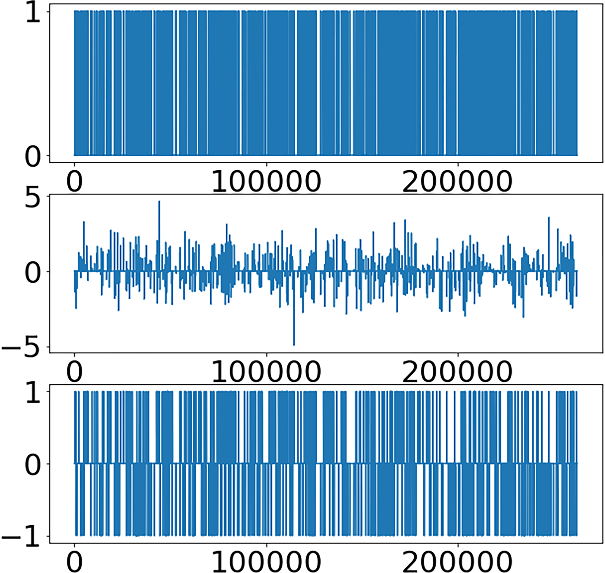
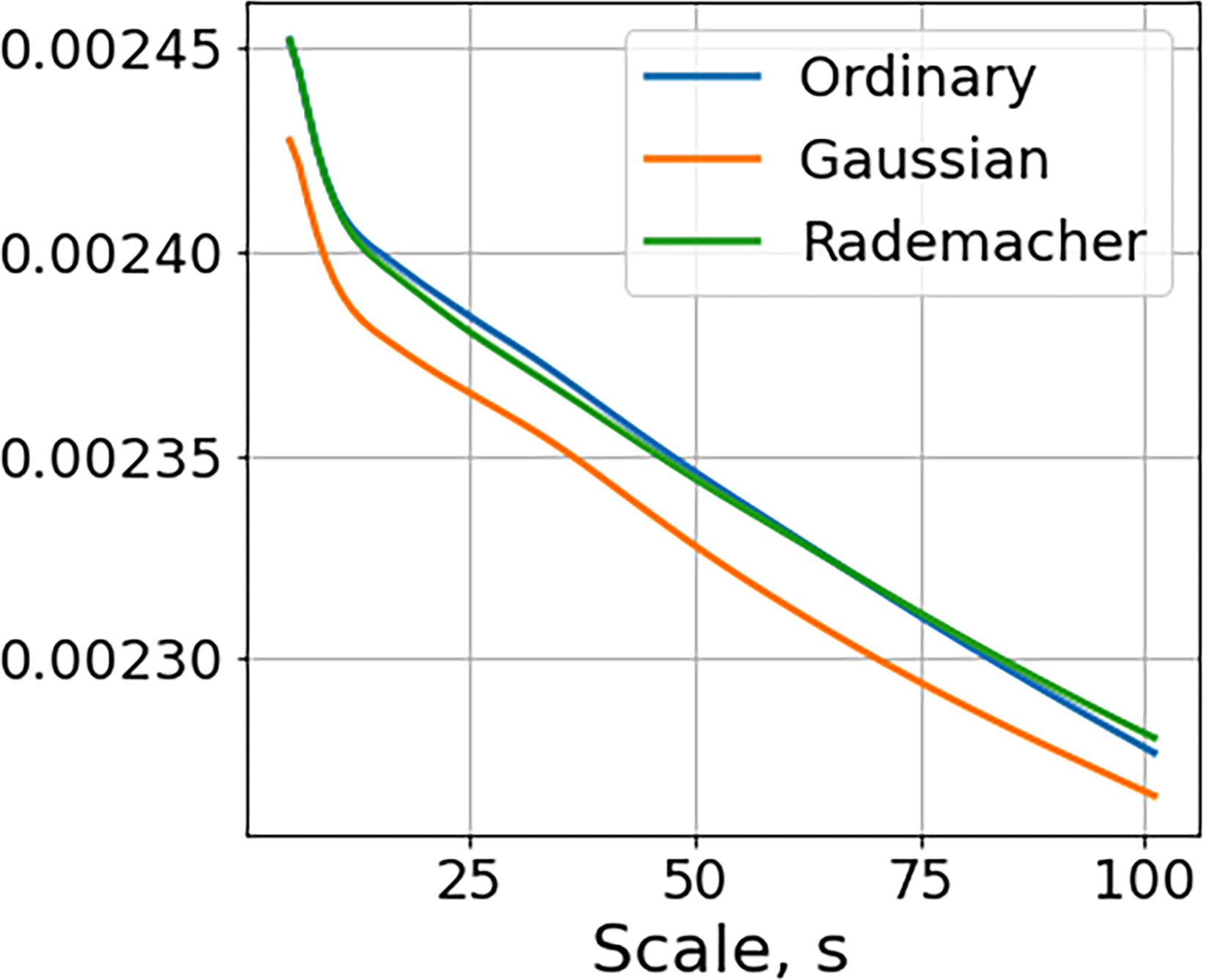
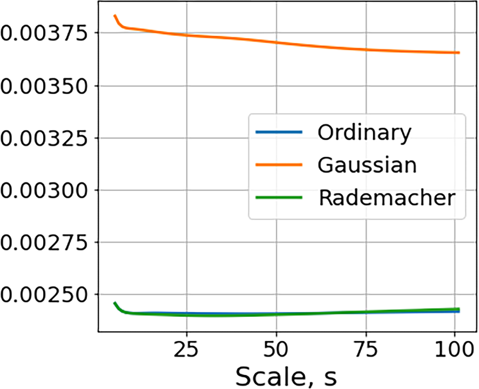
First-order invariant scattering moments of homogeneous compound Poisson point processes with the same intensity λ₀ and different A_i. Left: Realizations of the process with arrival rates given by Top: A_i = 1 Middle: A_i are normal random variables Bottom: A_i are Rademacher random variables. Middle: Plots of normalized first-order scattering $\frac{SY(s,\xi ,1)}{s\Vert w{\Vert }_1}$ moments with p = 1.Right: Plots of normalized first-order scattering $\frac{SY(s,\xi ,2)}{s\Vert w{\Vert }_2^2}$ moments with p = 2.

Inhomogeneous, non-compound Poisson point processes:

We also consider an inhomogeneous, non-compound Poisson point processes with intensity function $\lambda (t)=0.01\left(1+0.5\sin \left(\frac{2\pi t}{N}\right)\right)$ (where we estimate S_γ,pY(t), by averaging over 1000 realizations). Figure 2 plots the scattering moments for the inhomogeneous process at different times, and shows they align with the true intensity function.

Fig. 2.

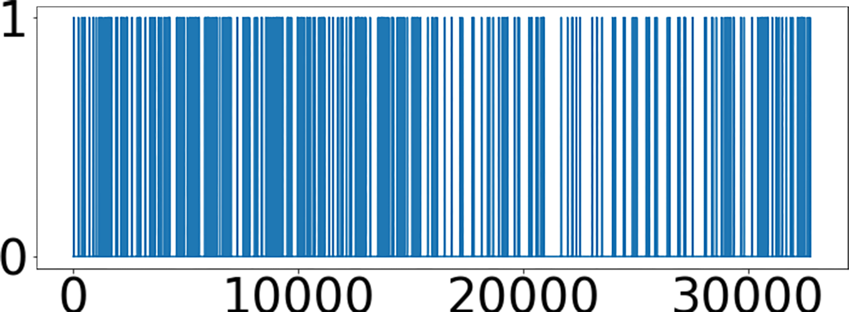
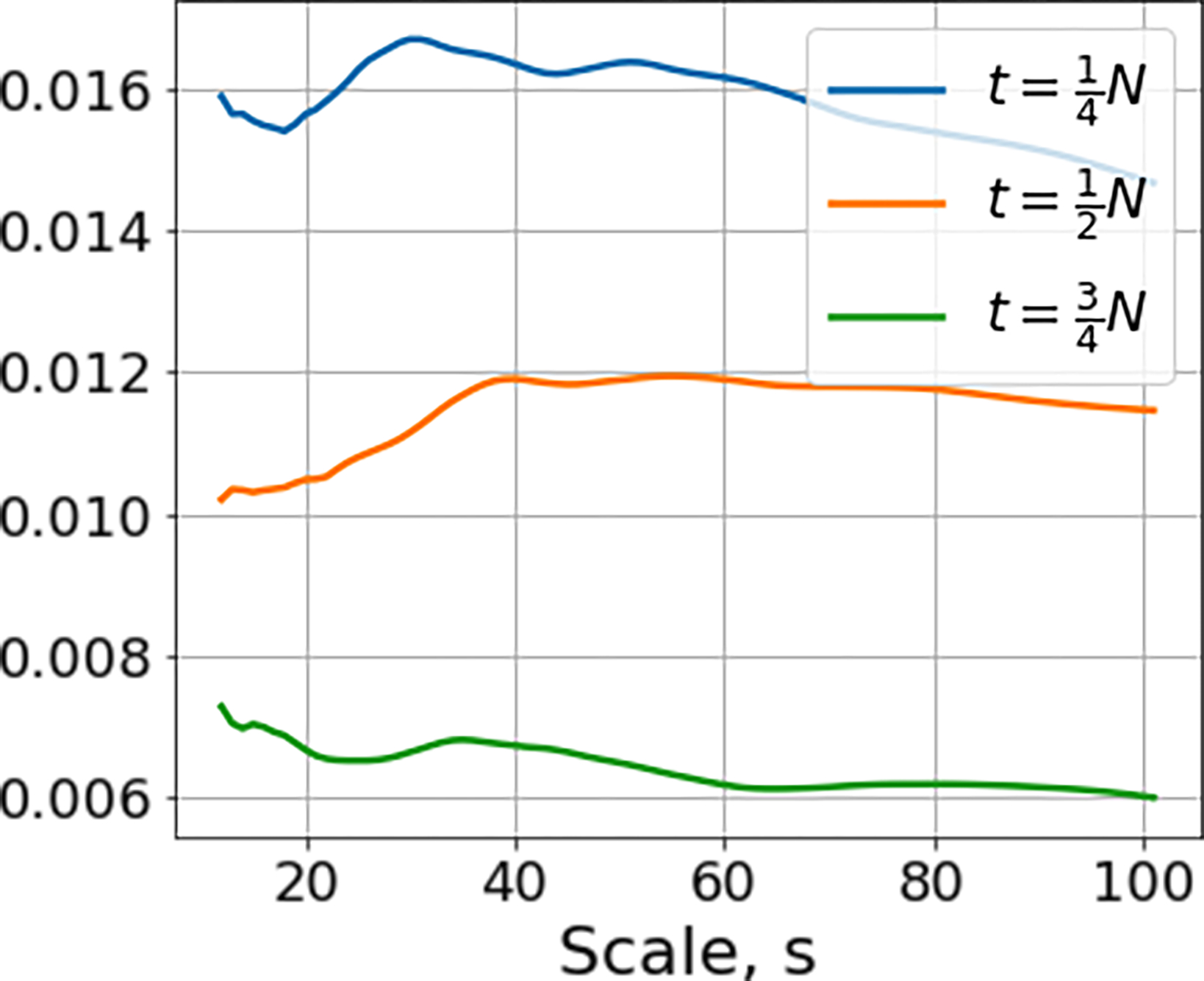
First-order scattering moments for inhomogeneous Poisson point processes. Left: Sample realization with $\lambda (t)=0.01\left(1+0.5\sin \left(\frac{2\pi t}{N}\right)\right)$. Right: Time-dependent scattering moments $\frac{S_{\gamma ,p}Y(t)}{s\Vert w{\Vert }_P^p}$ at $t_1=\frac{N}{4}$, $t_2=\frac{N}{2}$,$t_3=\frac{3N}{4}$. Note that the scattering coefficients at times t₁, t₂, t₃ converges to λ(t₁) = 0.015, λ(t₂) = 0.01, λ(t₃) = 0.005.

Poisson point process and self similar process:

We consider a Brownian motion compared to a Poisson point process with intensity λ = 0.01 and charges ${(A)}_{j=1}^{\infty }\equiv 10$. Figure 3 shows the convergence rate of the first-order scattering moments can distinguish these processes when p = 1 but not when p = 2.

Fig. 3.

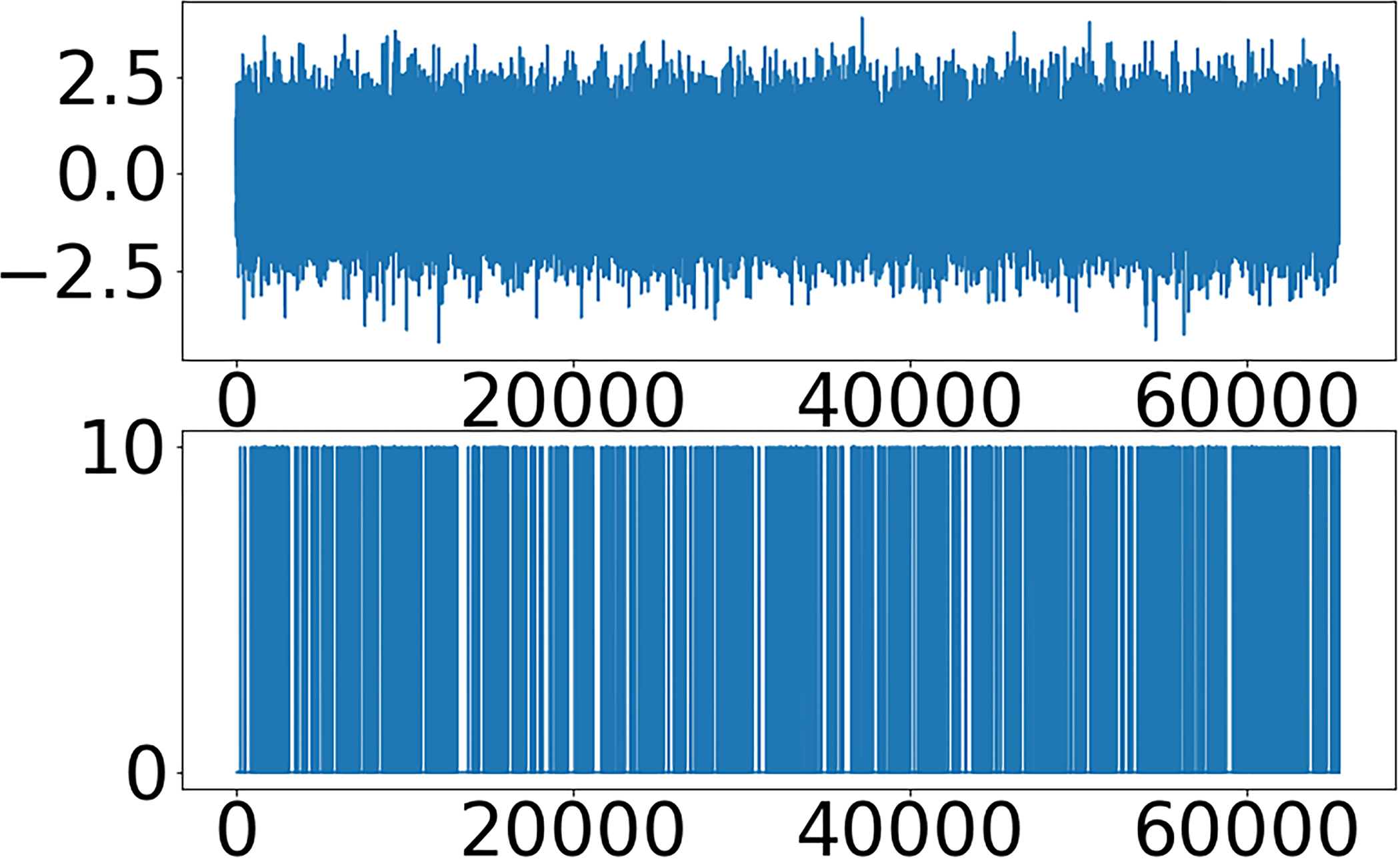
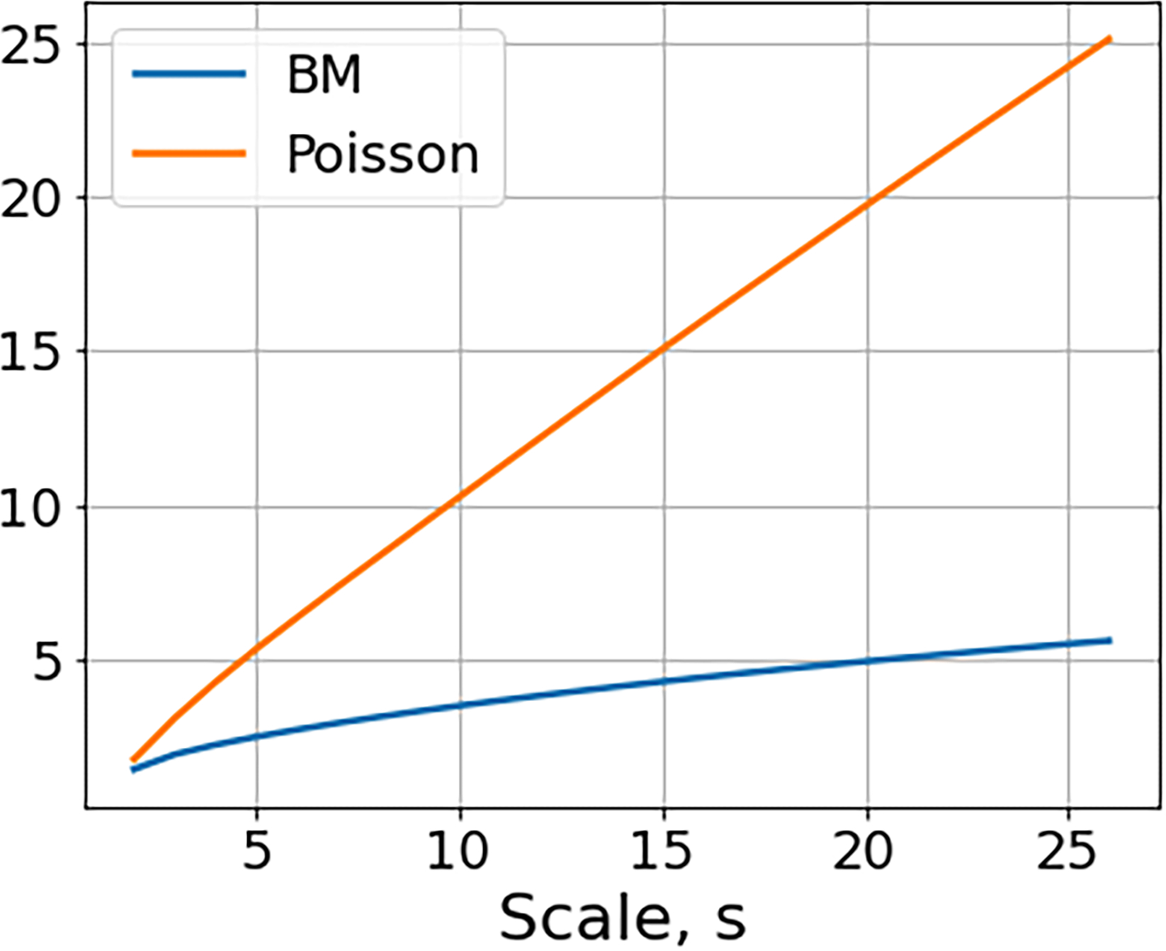
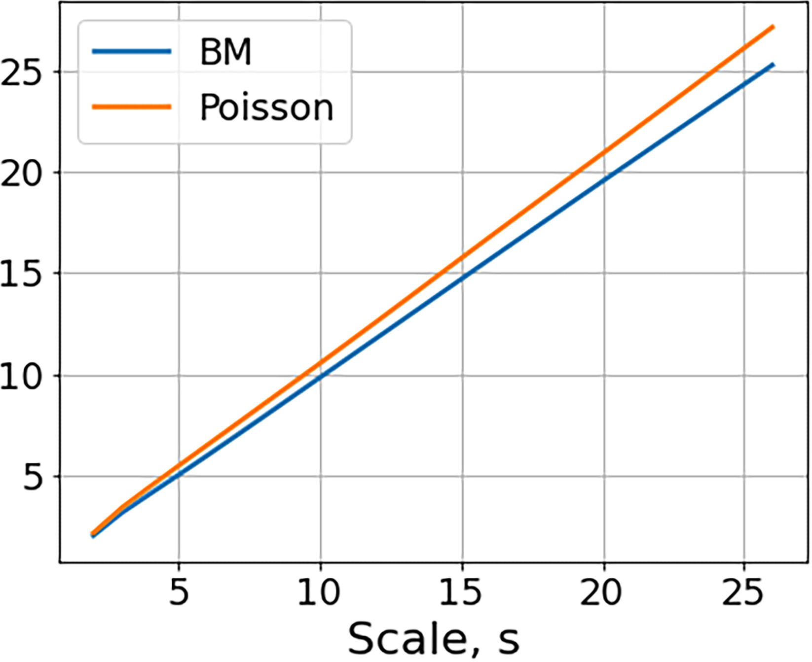
First-order invariant scattering moments for standard Brownian motion and Poisson point process. Left: Sample realizations Top: Brownian motion. Bottom: Ordinary Poisson point process. Middle: Normalized scattering moments $\frac{S{Y}_{\text{poisson}}(x,\xi ,p)}{\lambda \mathbb{E}{\left|A_1\right|}^p\Vert w{\Vert }_p^p}$ and $\frac{S{X}_{\text{BM}}(s,\xi ,p)}{\lambda \mathbb{E}|Z{|}^p\Vert w{\Vert }_p^p}$ for Poisson and BM with p = 1. Right: The same but with p = 2.

6. CONCLUSION

We have constructed Gabor-filter scattering transforms for random measures on ${ℝ}^d$. Our work is closely related to [14] but considers more general classes of filters and point processes (although we note that [14] provides a more detailed analysis of self-similar processes). In future work, it would be interesting to explore the use of these measurements for tasks such as, e.g., synthesizing new signals.

A. PROOF OF THEOREM 1

To prove Theorem 1 we will need the following lemma.

Lemma 1.

Let Z be a Poisson random variable with parameter λ. Then for all $\alpha \in ℝ$, $m\in \mathbb{N}$, 0 < λ < 1, we have

$$\mathbb{E}\left[Z^{\alpha }{1}_{\{Z>m\}}\right]=\sum _{k=m+1}^{\infty }{e}^{-\lambda }\frac{{\lambda }^k}{k!}{k}^{\alpha }⩽C_{m,\alpha }{\lambda }^{m+1}.$$

Proof. For 0 < λ < 1 and $k\in \mathbb{N}$, e^−λλ^k ⩽ 1. Therefore,

$$\begin{gathered} \mathbb{E}\left[Z^{\alpha }{\mathbb{1}}_{\{Z>m\}}\right]=\sum _{k=m+1}^{\infty }{e}^{-\lambda }\frac{{\lambda }^k}{k!}{k}^{\alpha } \\ ={\lambda }^{m+1}\sum _{k=0}^{\infty }{e}^{-\lambda }\frac{{\lambda }^k}{(k+m+1)!}{(k+m+1)}^{\alpha } \\ ⩽{\lambda }^{m+1}\sum _{k=0}^{\infty }\frac{{(k+m+1)}^{\alpha }}{(k+m+1)!} \\ =C_{\alpha ,m}{\lambda }^{m+1}. \end{gathered}$$

The proof of Theorem 1. Recalling the definitions of Y(dt) and S_γ,pY(t), and setting N_s(t) = N([t − s, t]^d), we see

$$\begin{gathered} S_{\gamma ,p}Y(t)=\mathbb{E}\left[{\left|{\int }_{{[s-t,t]}^d}w\left(\frac{t-u}{s}\right)e^{i\xi \cdot (t-u)}Y(du)\right|}^p\right] \\ =\mathbb{E}\left[{\left|\sum _{j=1}^{N_s(t)}{A}_{j}w\left(\frac{t-t_j}{s}\right)e^{i\xi \cdot \left(t-t_j\right)}\right|}^p\right], \end{gathered}$$

where $t_1,t_2,\dots t_{N_s(t)}$ are the points N(t) in [t − s, t]^d. Conditioned on the event that N_s(t) = k, the locations of the k points on [t − s, t]^d are distributed as i.i.d. random variables Z₁, . . . , Z_k taking values in [t − s, t]^d with density

$$p_Z(z)=\frac{\lambda (z)}{{\mathrm{\Lambda }}_s(t)},z\in {[t-s,t]}^d.$$

Therefore, the random variables

$$V_i:=\frac{t-Z_i}{s}$$

take values in the unit cube [0, 1]^d and have density

$$p_V(v)=\frac{s^d}{{\mathrm{\Lambda }}_s(t)}\lambda (t-vs),v\in {[0,1]}^d.$$

Note that in the special case that N is homogeneous, i.e. λ(t) ≡ λ₀ is constant, the V_i are uniform random variables on [0, 1]^d.

Therefore, computing the conditional expectation, we have for k ⩾ 1

$$\mathbb{E}\left[{\left|\sum _{j=1}^{N_s(t)}{A}_{j}w\left(\frac{t-t_j}{s}\right)e^{i\xi \cdot \left(t-t_j\right)}\right|}^p:N_s(t)=k\right]$$ (13)

$$=\mathbb{E}\left[{\left|\sum _{j=1}^k{A}_{j}w\left(V_j\right)e^{is\xi \cdot V_j}\right|}^p\right]$$

$$⩽\frac{\Vert \lambda {\Vert }_{\infty }}{{\lambda }_{\min }}{k}^p\mathbb{E}\left[{\left|A_1\right|}^p\right]\Vert w{\Vert }_p^p,$$ (14)

where (14) follows from (i) the independence of the random variables A_j and V_j; (ii) the fact that for any sequence of i.i.d. random variables Z₁, Z₂, . . .,

$$\mathbb{E}\left[{\left|\sum _{n=1}^k{Z}_n\right|}^p\right]⩽k^{p-1}\mathbb{E}\left[\sum _{n=1}^k{\left|Z_n\right|}^p\right]=k^p\mathbb{E}\left[{\left|Z_1\right|}^p\right];$$

and (iii) the fact that

$$\mathbb{E}\left[{\left|w\left(V_i\right)\right|}^p\right]={\int }_{{[0,1]}^d}|w(v){|}^p{p}_V(v)dv⩽\frac{\Vert \lambda {\Vert }_{\infty }}{{\lambda }_{\min }}\Vert w{\Vert }_p^p.$$

Therefore, since $\mathbb{P}\left[N_s(t)=k\right]=e^{-{\mathrm{\Lambda }}_s(t)}\cdot {\left({\mathrm{\Lambda }}_s(t)\right)}^k/k!$,

$$\mathbb{E}\left[{\left|\sum _{j=1}^{N_s(t)}{A}_{j}w\left(\frac{t-t_j}{s}\right)e^{i\xi \cdot \left(t-t_j\right)}\right|}^p\right]=$$

$$=\sum _{k=0}^{\infty }{e}^{-{\mathrm{\Lambda }}_s(t)}\frac{{\left({\mathrm{\Lambda }}_s(t)\right)}^k}{k!}\mathbb{E}\left[{\left|\sum _{j=1}^{N_s(t)}{A}_{j}w\left(\frac{t-t_j}{s}\right)e^{i\xi \cdot \left(t-t_j\right)}\right|}^p:N_s(t)=k\right]$$

$$=\sum _{k=1}^{\infty }{e}^{-{\mathrm{\Lambda }}_s(t)}\frac{{\left({\mathrm{\Lambda }}_s(t)\right)}^k}{k!}\mathbb{E}\left[{\left|\sum _{j=1}^k{A}_{j}w\left(V_j\right)e^{is\xi \cdot V_j}\right|}^p\right]$$

$$=\sum _{k=1}^m{e}^{-{\mathrm{\Lambda }}_s(t)}\frac{{\left({\mathrm{\Lambda }}_s(t)\right)}^k}{k!}\mathbb{E}\left[{\left|\sum _{j=1}^k{A}_{j}w\left(V_j\right)e^{is\xi \cdot V_j}\right|}^p\right]+\epsilon (m,s,\xi ,t),$$

where

$$\epsilon (m,s,t,\xi ):=\sum _{k=m+1}^{\infty }{e}^{-{\mathrm{\Lambda }}_s(t)}\frac{{\left({\mathrm{\Lambda }}_s(t)\right)}^k}{k!}\mathbb{E}\left[{\left|\sum _{j=1}^k{A}_{j}w\left(V_j\right)e^{is\xi \cdot V_j}\right|}^p\right].$$

By (14) and Lemma 1, if s is small enough so that Λ_s(t) ⩽ s^d∥λ∥_∞ < 1, then:

$$\begin{gathered} \epsilon (m,s,\xi ,t)=\sum _{k=m+1}^{\infty }{e}^{-{\mathrm{\Lambda }}_s(t)}\frac{{\left({\mathrm{\Lambda }}_s(t)\right)}^k}{k!}\mathbb{E}\left[{\left|\sum _{j=1}^k{A}_{j}w\left(V_j\right)e^{is\xi \cdot V_j}\right|}^p\right] \\ ⩽\frac{\Vert \lambda {\Vert }_{\infty }}{{\lambda }_{\min }}\mathbb{E}\left[{\left|A_1\right|}^p\right]\Vert w{\Vert }_p^p\sum _{k=m+1}^{\infty }{e}^{-{\mathrm{\Lambda }}_s(t)}\frac{{\left({\mathrm{\Lambda }}_s(t)\right)}^k}{k!}{k}^p \\ ⩽C_{m,p}\frac{\Vert \lambda {\Vert }_{\infty }}{{\lambda }_{\min }}\mathbb{E}\left[{\left|A_1\right|}^p\right]\Vert w{\Vert }_p^p{\left({\mathrm{\Lambda }}_s(t)\right)}^{m+1} \\ ⩽C_{m,p}\frac{\Vert \lambda {\Vert }_{\infty }}{{\lambda }_{\min }}\mathbb{E}\left[{\left|A_1\right|}^p\right]\Vert w{\Vert }_p^p\Vert \lambda {\Vert }_{\infty }^{m+1}{s}^{d(m+1)}. \end{gathered}$$

B. PROOF OF THEOREM 2

Proof. Let (s_k, ξ_k) be a sequence of scale and frequency pairs such that lim_k→∞ s_k = 0. Applying Theorem 1 with m = 1, we obtain:

$$\begin{gathered} \frac{S_{{\gamma }_k,p}Y(t)}{s_k^d} \\ =e^{-{\mathrm{\Lambda }}_{s_k}(t)}\frac{{\mathrm{\Lambda }}_{s_k}(t)}{s_k^d}\mathbb{E}\left[{\left|A_{1}w\left(V_{1,k}\right)e^{is\xi \cdot V_{1,k}}\right|}^p\right]+\frac{\epsilon \left(1,s_k,{\xi }_k,t\right)}{s_k^d} \\ =e^{-{\mathrm{\Lambda }}_{s_k}(t)}\frac{{\mathrm{\Lambda }}_{s_k}(t)}{s_k^d}\mathbb{E}\left[{\left|A_1\right|}^p\right]\mathbb{E}\left[{\left|w\left(V_{1,k}\right)\right|}^p\right]+\frac{\epsilon \left(1,s_k,{\xi }_k,t\right)}{s_k^d}, \end{gathered}$$

where we write V_1,k = V₁ to emphasize the fact that the density of V_1,k is:

$$p_{V_k}(v)=\frac{s_k^d}{{\mathrm{\Lambda }}_{s_k}(t)}\lambda \left(t-v{s}_k\right).$$

Using the error bound (7), we see that:

$$\underset{k\to \infty }{\lim }\frac{\epsilon \left(1,s_k,{\xi }_k,t\right)}{s_k^d}=0.$$

Furthermore, since $0⩽{\mathrm{\Lambda }}_{s_k}(t)⩽s_k^d\Vert \lambda {\Vert }_{\infty }$, we observe that:

$$\underset{k\to \infty }{\lim }{e}^{-{\mathrm{\Lambda }}_{s_k}(t)}=1,$$

and by the continuity of λ(t),

$$\underset{k\to \infty }{\lim }\frac{{\mathrm{\Lambda }}_{s_k}(t)}{s_k^d}=\underset{k\to \infty }{\lim }\frac{1}{s_k^d}{\int }_{{\left[s_k-t,t\right]}^d}\lambda (u)du=\lambda (t).$$ (15)

Finally, by the continuity of λ(t), we see that

$$p_{V_k}(v)⩽\frac{\Vert \lambda {\Vert }_{\infty }}{{\lambda }_{\min }}\text{and}\underset{k\to \infty }{\lim }{p}_{V_k}(v)=1,\forall v\in {[0,1]}^d\text{.}$$ (16)

Therefore, by the bounded convergence theorem,

$$\begin{gathered} \underset{k\to \infty }{\lim }\mathbb{E}\left[{\left|w\left(V_1\right)\right|}^p\right]=\underset{k\to \infty }{\lim }{\int }_{{[0,1]}^d}|w(v){|}^p{p}_{V_k}(v)dv \\ ={\int }_{{[0,1]}^d}|w(v){|}^p\underset{k\to \infty }{\lim }{p}_{V_k}(v)dv \\ =\Vert w{\Vert }_p^p. \end{gathered}$$

That completes the proof of (8).

To prove (9), we assume that λ(t) is periodic with period T along each coordinate and again use Theorem 1 with m = 1 to observe,

$$\begin{gathered} \frac{SY\left(s_k,{\xi }_k,p\right)}{s_k^d} \\ =\mathbb{E}\left[{\left|A_1\right|}^p\right]\frac{1}{T^d}{\int }_{{[0,T]}^d}{e}^{-{\mathrm{\Lambda }}_{s_k}(t)}\frac{{\mathrm{\Lambda }}_{s_k}(t)}{s_k^d}\times \\ {\int }_{{[0,1]}^d}|w(v){|}^p{p}_{V_k}(v)dvdt+\frac{1}{T^d}{\int }_{{[0,1]}^d}\frac{\epsilon \left(1,s_k,{\xi }_k,t\right)}{s_k^d}dt. \end{gathered}$$

By (7), the second integral converges to zero as k → 8. Therefore,

$$\underset{k\to \infty }{\lim }\frac{SY\left(s_k,{\xi }_k,p\right)}{s_k^d}=\mathbb{E}\left[{\left|A_1\right|}^p\right]\Vert w{\Vert }_p^p\frac{1}{T^d}{\int }_{{[0,T]}^d}\lambda (t)dt,$$

by the continuity of λ(t) and the bounded convergence theorem.

C. PROOF OF THEOREM 3

Proof. We apply Theorem 1 with m = 2 and obtain:

$$S_{{\gamma }_k,p}Y(t)$$ (17)

$$=e^{-{\mathrm{\Lambda }}_{s_k}(t)}{\mathrm{\Lambda }}_{s_k}(t)\mathbb{E}\left[{\left|A_1\right|}^p\right]\mathbb{E}\left[{\left|w\left(V_{1,k}\right)\right|}^p\right]$$ (18)

$$+e^{-{\mathrm{\Lambda }}_{s_k}(t)}\frac{{\left({\mathrm{\Lambda }}_{s_k}(t)\right)}^2}{2}\mathbb{E}\left[{\left|A_{1}w\left(V_{1,k}\right)e^{i{s}_k{\xi }_k\cdot V_{1,k}}+A_{2}w\left(V_{2,k}\right)e^{i{s}_k{\xi }_k\cdot V_{2,k}}\right|}^p\right]$$ (19)

$$+\epsilon \left(2,s_k,{\xi }_k,t\right),$$

where V_i,k, i = 1,2, are random variables taking values on the unit cube [0, 1]^d with densities,

$$p_{V_k}(v)=\frac{s_k^d}{{\mathrm{\Lambda }}_{s_k}(t)}\lambda \left(t-v{s}_k\right).$$

Dividing both sides in (18) by $s_k^{2d}\Vert w{\Vert }_p^p\mathbb{E}\left[{\left|A_1\right|}^p\right]$ and subtracting $\frac{{\mathrm{\Lambda }}_{s_k}(t)}{s_k^{2d}}\frac{\mathbb{E}\left[{\left|w\left(V_{1,k}\right)\right|}^p\right]}{\Vert w{\Vert }_p^p}$ yields:

$$\frac{S_{{\gamma }_k,p}Y(t)}{s_k^{2d}\Vert w{\Vert }_p^p\mathbb{E}\left[{\left|A_1\right|}^p\right]}-\frac{{\mathrm{\Lambda }}_{s_k}(t)}{s_k^{2d}}\frac{\mathbb{E}\left[{\left|w\left(V_{1,k}\right)\right|}^p\right]}{\Vert w{\Vert }_p^p}$$ (20)

$$=\frac{e^{-{\mathrm{\Lambda }}_{s_k}(t)}{\mathrm{\Lambda }}_{s_k}(t)-{\mathrm{\Lambda }}_{s_k}(t)}{s_k^{2d}}\frac{\mathbb{E}\left[{\left|w\left(V_{1,k}\right)\right|}^p\right]}{\Vert w{\Vert }_p^p}$$ (21)

$$+e^{-{\mathrm{\Lambda }}_{s_k}(t)}\frac{{\left({\mathrm{\Lambda }}_{s_k}(t)\right)}^2}{s_k^{2d}}\frac{\mathbb{E}\left[{\left|A_{1}w\left(V_{1,k}\right)e^{i{s}_k{\xi }_k\cdot V_{1,k}}+A_{2}w\left(V_{2,k}\right)e^{i{s}_k{\xi }_k\cdot V_{2,k}}\right|}^p\right]}{2\Vert w{\Vert }_p^p\mathbb{E}\left[{\left|A_1\right|}^p\right]}$$

$$+\frac{\epsilon \left(2,s_k,{\xi }_k,t\right)}{s_k^{2d}\Vert w{\Vert }_p^p\mathbb{E}\left[{\left|A_1\right|}^p\right]}.$$

Using the error bound (7),

$$\underset{k\to \infty }{\lim }\frac{\epsilon \left(2,s_k,{\xi }_k,t\right)}{s_k^{2d}\Vert w{\Vert }_p^p\mathbb{E}\left[{\left|A_1\right|}^p\right]}=0,$$ (22)

at a rate independent of t. Recalling (16) from the proof of Theorem 2, we use the fact that ${\lim }_{k\to \infty }{p}_{V_k}\equiv 1$ and the bounded convergence theorem to conclude,

$$\underset{k\to \infty }{\lim }\mathbb{E}\left[{|A_{1}w\left(V_{1,k}\right)e^{i{s}_k{\xi }_k\cdot V_{1,k}}+A_{2}w\left(V_{2,k}\right)e^{i{s}_k{\xi }_k\cdot V_{2,k}}|}^p\right]$$ (23)

$$=\mathbb{E}\left[{\left|A_{1}w\left(U_1\right)e^{iL\cdot U_1}+A_{2}w\left(U_2\right)e^{iL\cdot U_2}\right|}^p\right],$$ (24)

where U_i, i = 1, 2, are uniform random variables on the unit cube and $L={\lim }_{k\to \infty }{s}_k{\xi }_k$. Similarly,

$$\underset{k\to \infty }{\lim }\frac{\mathbb{E}\left[{\left|w\left(V_{1,k}\right)\right|}^p\right]}{\Vert w{\Vert }_p^p}=1.$$ (25)

Lastly, recalling that s_k → 0 as k → 8 and using (15) from the proof of Theorem 2, we see

$$\underset{k\to \infty }{\lim }\frac{e^{-{\mathrm{\Lambda }}_{s_k}(t)}{\mathrm{\Lambda }}_{s_k}(t)-{\mathrm{\Lambda }}_{s_k}(t)}{s_k^{2d}}$$ (26)

$$\begin{gathered} =\underset{k\to \infty }{\lim }\left(\frac{{\mathrm{\Lambda }}_{s_k}(t)}{s_k^d}\right)\underset{k\to \infty }{\lim }\left(\frac{e^{-{\mathrm{\Lambda }}_{s_k}(t)}-1}{s_k^d}\right) \\ =\lambda (t)\underset{k\to \infty }{\lim }\left(\frac{e^{-{\mathrm{\Lambda }}_{s_k}(t)}-1}{s_k^d}\right) \\ =-\lambda {(t)}^2. \end{gathered}$$ (27)

Now we integrate both sides of (21) over [0, T]^d and divide by T^d. Taking the limit as k → 8, on the left hand side we get:

$$\begin{gathered} \underset{k\to \infty }{\lim }\frac{1}{T^d}{\int }_{{[0,T]}^d}\left(\frac{S_{{\gamma }_k,p}Y(t)}{s_k^{2d}\Vert w{\Vert }_p^p\mathbb{E}\left[{\left|A_1\right|}^p\right]}-\frac{{\mathrm{\Lambda }}_{s_k}(t)}{s_k^{2d}}\frac{\mathbb{E}\left[{\left|w\left(V_{1,k}\right)\right|}^p\right]}{\Vert w{\Vert }_p^p}\right)dt \\ =\underset{k\to \infty }{\lim }\left(\frac{SY\left(s_k,{\xi }_k,p\right)}{s_k^{2d}\Vert w{\Vert }_p^p\mathbb{E}\left[{\left|A_1\right|}^p\right]}-\frac{\mathbb{E}\left[{\left|w\left(V_{1,k}\right)\right|}^p\right]}{\Vert w{\Vert }_p^p{T}^d}{\int }_{{[0,T]}^d}\frac{{\mathrm{\Lambda }}_{s_k}(t)}{s_k^{2d}}dt\right) \\ =\underset{k\to \infty }{\lim }\left(\frac{SY\left(s_k,{\xi }_k,p\right)}{s_k^{2d}\mathbb{E}\left[{\left|w\left(V_{1,k}\right)\right|}^p\right]\mathbb{E}\left[{\left|A_1\right|}^p\right]}-\frac{1}{T^d}{\int }_{{[0,T]}^d}\frac{{\mathrm{\Lambda }}_{s_k}(t)}{s_k^{2d}}dt\right), \end{gathered}$$

where we used the definition of the invariant scattering moments and (25). On the right hand side of (21), we use (25), (27) and the dominated convergence theorem to see that the first term is:

$$\begin{gathered} \underset{k\to \infty }{\lim }\frac{1}{T^d}{\int }_{{[0,T]}^d}\frac{e^{-{\mathrm{\Lambda }}_{s_k}(t)}{\mathrm{\Lambda }}_{s_k}(t)-{\mathrm{\Lambda }}_{s_k}(t)}{s_k^{2d}}\frac{\mathbb{E}\left[{\left|w\left(V_{1,k}\right)\right|}^p\right]}{\Vert w{\Vert }_p^p}dt \\ =\underset{k\to \infty }{\lim }\frac{1}{T^d}{\int }_{{[0,T]}^d}\frac{e^{-{\mathrm{\Lambda }}_{s_k}(t)}{\mathrm{\Lambda }}_{s_k}(t)-{\mathrm{\Lambda }}_{s_k}(t)}{s_k^{2d}}dt \\ =-\frac{1}{T^d}{\int }_{{[0,T]}^d}\lambda {(t)}^{2}dt. \end{gathered}$$

Using (15), (23), and the bounded convergence theorem, the second term of (21) is:

$$\begin{gathered} \underset{k\to \infty }{\lim }\frac{1}{T^d}{\int }_{{[0,T]}^d}{e}^{-{\Lambda }_{s_k}(t)}{X}_{k}dt \\ =\frac{\mathbb{E}\left[\mid A_{1}w\left(U_1\right)e^{iL\cdot U_1}+A_{2}w\left(U_2\right)e^{\left.{\left.iL\cdot U_2\right|}^p\right]}\right.}{2T^d\Vert w{\Vert }_p^p\mathbb{E}\left[|A_1{|}^p\right]}\left({\int }_{{[0,T]}^d}\lambda {(t)}^{2}dt\right) \end{gathered}$$

where

$$X_k=\frac{\mathbb{E}\left[{\left|A_{1}w\left(V_{1,k}\right)e^{i{s}_k{\xi }_k\cdot V_{1,k}}+A_{2}w\left(V_{2,k}\right)e^{i{s}_k{\xi }_k\cdot V_{2,k}}\right|}^p\right]}{2\Vert w{\Vert }_p^p\mathbb{E}\left[{\left|A_1\right|}^p\right]}.$$

Finally, the third term of (21) goes to zero using the bounded convergence theorem and (22). Putting together the left and right hand sides of (21) with these calculations finishes the proof.

D. PROOF OF THEOREM 4

Proof. As in the proof of Theorem 1, let N_s(t) = N ([t − s, t]^d) denote the number of points in the cube [t − s, t]^d. Then since the support of w is contained in [0, 1]^d,

$$\begin{gathered} \left(g_{{\gamma }_k}*Y\right)(t)={\int }_{{\left[t-s_k,t\right]}^d}w\left(\frac{t-u}{s_k}\right)e^{i{\xi }_k\cdot (t-u)}Y(du) \\ =\sum _{j=1}^{N_{s_k}(t)}{A}_{j}w\left(\frac{t-t_j}{s_k}\right)e^{i{\xi }_k\cdot \left(t-t_j\right)}, \end{gathered}$$

where $t_1,t_2,\dots ,t_{N_{s_k}}(t)$ are the points of N in [t − s_k, t]^d. Therefore, in the event that $N_{s_k}(t)=1$,

$${\left|\left(g_{{\gamma }_k}*Y\right)(t)\right|}^p=\left({\left|g_{{\gamma }_k}\right|}^p*|Y{|}^p\right)(t),$$

and so, partitioning the space of possible outcomes based on $N_{s_k}\text{(}t\text{)}$, we obtain:

$$\begin{gathered} {\left|\left(g_{{\gamma }_k}*Y\right)(t)\right|}^p \\ ={\left|\left(g_{{\gamma }_k}*Y\right)(t)\cdot {\mathbb{1}}_{\left\{N_{s_k}(t)=1\right\}}+\left(g_{{\gamma }_k}*Y\right)(t)\cdot {\mathbb{1}}_{\left\{N_{s_k}(t)>1\right\}}\right|}^p \\ ={\left|\left(g_{{\gamma }_k}*Y\right)(t)\cdot {\mathbb{1}}_{\left\{N_{s_k}(t)=1\right\}}\right|}^p+{\left|\left(g_{{\gamma }_k}*Y\right)(t)\cdot {\mathbb{1}}_{\left\{N_{s_k}(t)>1\right\}}\right|}^p \\ =\left({\left|g_{{\gamma }_k}\right|}^p*|Y{|}^p\right)(t)\cdot {\mathbb{1}}_{\left\{N_{s_k}(t)=1\right\}}+{\left|\left(g_{{\gamma }_k}*Y\right)(t)\cdot {\mathbb{1}}_{\left\{N_{s_k}(t)>1\right\}}\right|}^p \\ =\left({\left|g_{{\gamma }_k}\right|}^p*|Y{|}^p\right)(t)+e_k(t), \end{gathered}$$

where

$$e_k(t):={\left|\left(g_{{\gamma }_k}*Y\right)(t)\cdot {\mathbb{1}}_{\left\{N_{s_k}(t)>1\right\}}\right|}^p-\left({\left|g_{{\gamma }_k}\right|}^p*|Y{|}^p\right)(t)\cdot {\mathbb{1}}_{\left\{N_{s_k}(t)>1\right\}}$$

Using the above, we can write the second order convolution term as:

$$\left(g_{{\gamma }_k^{\prime }}*\left|g_{{\gamma }_k}*Y\right|\right)(t)=\left(g_{{\gamma }_k^{\prime }}*{\left|g_{{\gamma }_k}\right|}^p*|Y{|}^p\right)(t)+\left(g_{{\gamma }_k^{\prime }}*e_k\right)(t).$$

The following lemma implies that $\left(g_{{\gamma }_k^{\prime }}*e_k\right)(t)$ decays rapidly in ${\mathbf{L}}^{p^{\prime }}$ at a rate independent of t.

Lemma 2.

There exists δ > 0, independent of t, such that if s_k < δ,

$$\mathbb{E}\left[{\left|\left(g_{{\gamma }_k^{\prime }}*e_k\right)(t)\right|}^p\right]⩽C\left(p,p^{\prime },w,c,L\right)\frac{\Vert \lambda {\Vert }_{\infty }}{{\lambda }_{\min }}\Vert \lambda {\Vert }_{\infty }^2{s}_k^{d\left(p^{\prime }+2\right)}.$$

Once we have proved Lemma 2, equation (11) will follow once we show,

$$\underset{k\to \infty }{\lim }\frac{\mathbb{E}\left[{\left|\left(g_{{\gamma }_k^{\prime }}*{\left|g_{{\gamma }_k}\right|}^p*|Y{|}^p\right)(t)\right|}^{p^{\prime }}\right]}{s_k^{d\left(p^{\prime }+1\right)}}=K\left(p,p^{\prime },w,c,L\right)\lambda (t)\mathbb{E}\left[{\left|A_1\right|}^q\right].$$ (28)

Let us prove (28) first and postpone the proof of Lemma 2. We will use the fact that the support of $g_{{\gamma }_k^{\prime }}*{\left|g_{{\gamma }_k}\right|}^p$ is contained in ${\left[0,s_k+s_k^{\prime }\right]}^d$. Let ${\tilde{s}}_k:=s_k+s_k^{\prime }$, $N_k(t):=N_{{\overline{s}}_k}(t)$, ${\mathrm{\Lambda }}_k(t):={\mathrm{\Lambda }}_{{\overline{s}}_k}(t)$, and let $t_1,t_2,\dots ,t_{N_k(t)}$ be the points of N in the cube ${\left[t-{\tilde{s}}_k,t\right]}^d$. We have that $\mathbb{P}\left[N_k(t)=n\right]=e^{-{\mathrm{\Lambda }}_k(t)}\frac{{\left({\mathrm{\Lambda }}_k(t)\right)}^n}{n!}$, and conditioned on the event that N_k(t) = n, the locations of the points t₁, . . . , t_n are distributed as i.i.d. random variables Z₁(t), . . . , Z_n(t) taking values in ${\left[t-{\tilde{s}}_k,t\right]}^d$ with density $p_{Z(t)}(z)=\frac{\lambda (z)}{{\mathrm{\Lambda }}_k(t)}$. Therefore the i.i.d. random variables ${\tilde{V}}_1(t),\dots ,{\tilde{V}}_n(t)$ defined by ${\tilde{V}}_i(t):=t-Z_i(t)$ take values in ${\left[0,{\tilde{s}}_k\right]}^d$ and have density

$$p_{\tilde{V}(t)}(v)=\frac{\lambda (t-v)}{{\mathrm{\Lambda }}_k(t)},v\in {\left[0,{\tilde{s}}_k\right]}^d.$$

Now, we condition on N_k(t) to see that

$$\mathbb{E}\left[{\left|\left(g_{{\gamma }_k^{\prime }*}{\left|g_{{\gamma }_k}\right|}^p*|Y{|}^p\right)(t)\right|}^{p^{\prime }}\right]$$ (29)

$$=\mathbb{E}\left[{\left|\sum _{j=1}^{N_k(t)}{\left|A_j\right|}^p\left(g_{{\gamma }_k^{\prime }}*{\left|g_{{\gamma }_k}\right|}^p\right)\left(t-t_j\right)\right|}^{p^{\prime }}\right]$$

$$=\sum _{n=1}^{\infty }{e}^{-{\mathrm{\Lambda }}_k(t)}\frac{{\left({\mathrm{\Lambda }}_k(t)\right)}^n}{n!}$$ (30)

$$\cdot \mathbb{E}\left[{\left|\sum _{j=1}^{N_k(t)}{\left|A_j\right|}^p\left(g_{{\gamma }_k^{\prime }*}{\left|g_{{\gamma }_k}\right|}^p\right)\left(t-t_j\right)\right|}^{p^{\prime }}\text{:}{N}_k(t)=n\right]$$

$$=\sum _{n=1}^{\infty }{e}^{-{\mathrm{\Lambda }}_k(t)}\frac{{\left({\mathrm{\Lambda }}_k(t)\right)}^n}{n!}\mathbb{E}\left[{\left|\sum _{j=1}^n{\left|A_j\right|}^p\left(g_{{\gamma }_k^{\prime }*}{\left|g_{{\gamma }_k}\right|}^p\right)\left({\tilde{V}}_j(t)\right)\right|}^{p^{\prime }}\right]$$

$$=e^{-{\mathrm{\Lambda }}_k(t)}{\mathrm{\Lambda }}_k(t)\mathbb{E}\left[{\left|A_1\right|}^q\right]\mathbb{E}\left[{\left|\left(g_{{\gamma }_k^{\prime }}*{\left|g_{{\gamma }_k}\right|}^p\right)\left({\tilde{V}}_1(t)\right)\right|}^{p^{\prime }}\right]$$ (31)

$$+\sum _{n=2}^{\infty }{e}^{-{\mathrm{\Lambda }}_k(t)}\frac{{\left({\mathrm{\Lambda }}_k(t)\right)}^n}{n!}\mathbb{E}\left[{\left|{\sum _{j=1}^n\left|A_j\right|}^p\left(g_{{\gamma }_k^{\prime }}*{\left|g_{{\gamma }_k}\right|}^p\right)\left({\tilde{V}}_j(t)\right)\right|}^{p\prime }\right]$$ (32)

The following lemma will be used to estimate the scaling of the term in (31).

Lemma 3.

For all $t\in {ℝ}^d$,

$$\underset{k\to \infty }{\lim }\frac{{\tilde{s}}_k^d}{s_k^{d\left(p^{\prime }+1\right)}}\mathbb{E}\left[{\left|\left(g_{{\gamma }_k^{\prime }}*{\left|g_{{\gamma }_k}\right|}^p\right)\left({\tilde{V}}_1(t)\right)\right|}^{p^{\prime }}\right]={‖g_{c,L/c}*{\left|g_{1,0}\right|}^p‖}_{p^{\prime }}^{p^{\prime }}.$$ (33)

Furthermore, there exists δ > 0, independent of t, such that if s_k < δ then

$$\frac{{\tilde{s}}_k^d}{s_k^{d\left(p^{\prime }+1\right)}}\mathbb{E}\left[{\left|\left(g_{{\gamma }_k^{\prime }}*{\left|g_{{\gamma }_k}\right|}^p\right)\left({\tilde{V}}_1(t)\right)\right|}^{p^{\prime }}\right]⩽2\frac{\Vert \lambda {\Vert }_{\infty }}{{\lambda }_{\min }}C\left(p,p^{\prime },w,c,L\right).$$ (34)

Proof. Making a change of variables in both u and v, and recalling the assumption that $s_k^{\prime }=c{s}_k$, we observe that

$$\begin{gathered} \frac{{\tilde{s}}_k^d}{s_k^{d\left(p^{\prime }+1\right)}}\mathbb{E}\left[{\left|\left(g_{{\gamma }_k^{\prime }*}{\left|g_{{\gamma }_k}\right|}^p\right)\left({\tilde{V}}_1(t)\right)\right|}^{p^{\prime }}\right] \\ =\frac{{\tilde{s}}_k^d}{s_k^{d\left(p^{\prime }+1\right)}}{\int }_{{ℝ}^d}{p}_{\tilde{V}(t)}(v). \end{gathered}$$ (35)

$$\begin{gathered} {\left.{\left.\left|{\int }_{{ℝ}^d}w\left(\frac{v-u}{s_k^{\prime }}\right)e^{i{\xi }_k^{\prime }\cdot (v-u)}\right|w\left(\frac{u}{s_k}\right)\right|}^{p}du\right|}^{p^{\prime }}dv \\ ={\left.{\left.{\tilde{s}}_k^d{\int }_{{ℝ}^d}{p}_{\tilde{V}(t)}\left(s_{k}v\right)\left|{\int }_{{ℝ}^d}w\left(\frac{s_k(v-u)}{s_k^{\prime }}\right)e^{i{s}_k{\xi }_k^{\prime }\cdot (v-u)}\right|w(u)\right|}^{p}du\right|}^{p^{\prime }}dv \\ ={\left.{\left.{\int }_{{ℝ}^d}\frac{{\tilde{s}}_k^d\lambda \left(t-s_{k}v\right)}{{\mathrm{\Lambda }}_k(t)}\left|{\int }_{{ℝ}^d}w\left(\frac{u-v}{c}\right)e^{i{s}_k^{\prime }{\xi }_k^{\prime }\cdot (u-v)/c}\right|w(u)\right|}^{p}du\right|}^{p^{\prime }}dv. \end{gathered}$$ (36)

The continuity of λ(t) implies that

$$\underset{k\to \infty }{\lim }\frac{{\tilde{s}}_k^d\lambda \left(t-s_{k}v\right)}{{\mathrm{\Lambda }}_k(t)}=1,\forall v\in {[0,1+c]}^d.$$

Furthermore, the assumption 0 < λ_min ⩽ ∥λ∥_∞ < ∞ implies

$$\frac{{\tilde{s}}_k^d\lambda \left(t-s_{k}v\right)}{{\mathrm{\Lambda }}_k(t)}⩽\frac{\Vert \lambda {\Vert }_{\infty }}{{\lambda }_{\min }},\forall k⩾1.$$ (37)

Therefore, (33) follows from the dominated convergence theorem and by the observation that the inner integral of (36) is zero unless v ∈ [0, 1 + c]^d. Equation (34) follows from inserting (37) into (36) and sending k to infinity.

Since

$$\underset{k\to \infty }{\lim }\frac{{\mathrm{\Lambda }}_k(t)}{{\tilde{s}}_k^d}=\lambda (t),$$

the independence of ${\tilde{V}}_1(t)$ and A₁, the continuity of λ(t), and Lemma 3 imply that taking k → ∞ in (31) yields:

$$\begin{gathered} \underset{k\to \infty }{\lim }\left(\frac{e^{-{\mathrm{\Lambda }}_k(t)}{\mathrm{\Lambda }}_k(t)\mathbb{E}\left[{\left|A_1\right|}^q\right]\mathbb{E}\left[{\left.{\left.\left|g_{{\gamma }_k^{\prime }*}\right|g_{{\gamma }_k}\right|}^p\left({\tilde{V}}_1(t)\right)\right|}^{p^{\prime }}\right]}{s_k^{d\left(p^{\prime }+1\right)}}\right) \\ =\underset{k\to \infty }{\lim }\left(e^{-{\mathrm{\Lambda }}_k(t)}\frac{{\mathrm{\Lambda }}_k(t)}{{\tilde{s}}_k^d}\mathbb{E}\left[{\left|A_1\right|}^q\right]\frac{{\tilde{s}}_k^d}{s_k^{d\left(p^{\prime }+1\right)}}\mathbb{E}\left[{\left.{\left.\left|g_{{\gamma }_k^{\prime }}*\right|g_{{\gamma }_k}\right|}^p\left({\tilde{V}}_1(t)\right)\right|}^{p^{\prime }}\right]\right) \\ =K\left(p,p^{\prime },c,w,L\right)\lambda (t)\mathbb{E}\left[{\left|A_1\right|}^q\right]. \end{gathered}$$

The following lemma shows that (32) is $O\left(s_k^{d\left(p^{\prime }+2\right)}\right)$ (and converges at a rate independent of t), and therefore completes the proof of (11) subject to proving Lemma 2.

Lemma 4.

For all $\alpha \in ℝ$ there exists δ > 0, independent of t, such that if s_k < δ, then

$$\begin{gathered} \sum _{n=2}^{\infty }{e}^{-{\mathrm{\Lambda }}_k(t)}\frac{{\left({\mathrm{\Lambda }}_k(t)\right)}^n}{n!}{n}^{\alpha }\mathbb{E}\left[{\left|\sum _{j=1}^n{\left|A_j\right|}^p\left(g_{{\gamma }_k^{\prime }*}{\left|g_{{\gamma }_k}\right|}^p\right)\left({\tilde{V}}_j(t)\right)\right|}^{p^{\prime }}\right] \\ ⩽C\left(p,p^{\prime },w,c,\alpha ,L\right)\frac{\Vert \lambda {\Vert }_{\infty }}{{\lambda }_{\min }}\Vert \lambda {\Vert }_{\infty }^2\mathbb{E}\left[{\left|A_1\right|}^q\right]s_k^{d\left(p^{\prime }+2\right)}. \end{gathered}$$

Proof. For any sequence of i.i.d. random variables, Z₁, Z₂, . . . , it holds that

$$\mathbb{E}\left[{\left|\sum _{n=1}^k{Z}_n\right|}^p\right]⩽k^{p-1}\mathbb{E}\left[\sum _{n=1}^k{\left|Z_n\right|}^p\right]=k^p\mathbb{E}\left[{\left|Z_1\right|}^p\right].$$

Therefore, by Lemma 1, Lemma 3, and the fact that the ${\tilde{V}}_j(t)$ and A_i are i.i.d. and independent of each other, we see that if s_k < δ, where δ is as in (34),

$$\sum _{n=2}^{\infty }{e}^{-{\mathrm{\Lambda }}_k(t)}\frac{{\left({\mathrm{\Lambda }}_k(t)\right)}^n}{n!}{n}^{\alpha }$$

$$\times \mathbb{E}\left[{\left|\sum _{j=1}^n{\left|A_j\right|}^p\left(g_{{\gamma }_k^{\prime }*}{\left|g_{{\gamma }_k}\right|}^p\right)\left({\tilde{V}}_j(t)\right)\right|}^{p^{\prime }}\right]$$

$$⩽\sum _{n=2}^{\infty }{e}^{-{\mathrm{\Lambda }}_k(t)}\frac{{\left({\mathrm{\Lambda }}_k(t)\right)}^n}{n!}{n}^{\alpha }{n}^{p^{\prime }}$$

$$\times \mathbb{E}\left[{\left|A_1\right|}^q{\left|\left(g_{{\gamma }_k^{\prime }}*{\left|g_{{\gamma }_k}\right|}^p\right)\left({\tilde{V}}_1(t)\right)\right|}^{p^{\prime }}\right]$$

$$=\sum _{n=2}^{\infty }{e}^{-{\mathrm{\Lambda }}_k(t)}\frac{{\left({\mathrm{\Lambda }}_k(t)\right)}^n}{n!}{n}^{p^{\prime }+\alpha }$$

$$\times \mathbb{E}\left[{\left|A_1\right|}^q\right]\mathbb{E}\left[{\left|\left(g_{{\gamma }_k^{\prime }}*{\left|g_{{\gamma }_k}\right|}^p\right)\left({\tilde{V}}_1(t)\right)\right|}^{p^{\prime }}\right]$$

$$=\mathbb{E}\left[{\left|A_1\right|}^q\right]\mathbb{E}\left[{\left|\left(g_{{\gamma }_k^{\prime }}*{\left|g_{{\gamma }_k}\right|}^p\right)\left({\tilde{V}}_1(t)\right)\right|}^{p^{\prime }}\right]$$

$$\times \sum _{n=2}^{\infty }{e}^{-{\mathrm{\Lambda }}_k(t)}\frac{{\left({\mathrm{\Lambda }}_k(t)\right)}^n}{n!}{n}^{p^{\prime }+\alpha }$$

$$⩽C\left(p,p^{\prime },w,c,L\right)\frac{\Vert \lambda {\Vert }_{\infty }}{{\lambda }_{\min }}\mathbb{E}\left[{\left|A_1\right|}^q\right]\frac{s_k^{d\left(p^{\prime }+1\right)}}{{\tilde{s}}_k^d}$$

$$\times \sum _{n=2}^{\infty }{e}^{-{\mathrm{\Lambda }}_k(t)}\frac{{\left({\mathrm{\Lambda }}_k(t)\right)}^n}{n!}{n}^{p^{\prime }+\alpha }$$

$$⩽C\left(p,p^{\prime },w,c,L,\alpha \right)\frac{\Vert \lambda {\Vert }_{\infty }}{{\lambda }_{\min }}\mathbb{E}\left[{\left|A_1\right|}^q\right]\frac{s_k^{d\left(p^{\prime }+1\right)}}{{\tilde{s}}_k^d}{\left({\mathrm{\Lambda }}_k(t)\right)}^2$$

$$⩽C\left(p,p^{\prime },w,c,L,\alpha \right)\frac{\Vert \lambda {\Vert }_{\infty }}{{\lambda }_{\min }}\Vert \lambda {\Vert }_{\infty }^2\mathbb{E}\left[{\left|A_1\right|}^q\right]s_k^{d\left(p^{\prime }+2\right)},$$

where the last inequality uses the fact that ${\mathrm{\Lambda }}_k(t)⩽{\tilde{s}}_k^d\Vert \lambda {\Vert }_{\infty }={(1+c)}^d{s}_k^d\Vert \lambda {\Vert }_{\infty }$.

We will now complete the proof of the theorem by proving Lemma 2.

Proof. [Lemma 2] Since

$$\begin{gathered} e_k\text{(}t\text{)} \\ ={\left|\left(g_{{\gamma }_k}*Y\right)(t){\mathbb{1}}_{\left\{N_{s_k}(t)>1\right\}}\right|}^p-\left({\left|g_{{\gamma }_k}\right|}^p*|Y{|}^p\right)(t){\mathbb{1}}_{\left\{N_{s_k}(t)>1\right\}}, \end{gathered}$$

we see that

$$\begin{gathered} \left|g_{{\gamma }_k^{\prime }}*e_k(t)\right|⩽\left|g_{{\gamma }_k^{\prime }}*\left({\left|\left(g_{{\gamma }_k}*Y\right){\mathbb{1}}_{\left\{N_{s_k}(\cdot )>1\right\}}\right|}^p\right)(t)\right| \\ +\left|g_{{\gamma }_k^{\prime }}*\left(\left({\left|g_{{\gamma }_k}\right|}^p*|Y{|}^p\right){\mathbb{1}}_{\left\{N_{s_k}(\cdot )>1\right\}}\right)(t)\right|. \end{gathered}$$

First turning our attention to the second term, we note that

$$\begin{gathered} \left|g_{{\gamma }_k^{\prime }}*\left(\left({\left|g_{{\gamma }_k}\right|}^p*|Y{|}^p\right){\mathbb{1}}_{\left\{N_{s_k}(\cdot )>1\right\}}\right)(t)\right| \\ =\left|{\int }_{{\left[t-s_k^{\prime },t\right]}^d}w\left(\frac{t-u}{s_k^{\prime }}\right)e^{i{\xi }_k^{\prime }\cdot (t-u)}\left({\left|g_{{\gamma }_k}\right|}^p*|Y{|}^p\right)(u){\mathbb{1}}_{\left\{N_{s_k}(u)>1\right\}}du\right| \\ ⩽{\mathbb{1}}_{\left\{N_k(t)>1\right\}}{\int }_{{\left[t-s_k^{\prime },t\right]}^d}w\left(\frac{t-u}{s_k^{\prime }}\right)\left({\left|g_{{\gamma }_k}\right|}^p*|Y{|}^p\right)(u)du \\ ={\mathbb{1}}_{\left\{N_k(t)>1\right\}}\left(g_{s_k^{\prime },0}*{\left|g_{{\gamma }_k}\right|}^p*|Y{|}^p\right)(t). \end{gathered}$$ (38)

since $N_{s_k}(u)⩽N_{s_k+s_k^{\prime }}(t)=N_{{\overline{s}}_k}(t)=N_k(t)$ for all $u\in {\left[t-s_k^{\prime },t\right]}^d$. Therefore, conditioning on N_k(t), if s_k < δ,

$$\mathbb{E}\left[{\left|g_{{\gamma }_k^{\prime }*}\left(\left({\left|g_{{\gamma }_k}\right|}^p*|Y{|}^p\right){\mathbb{1}}_{\left\{N_{s_k}(\cdot )>1\right\}}\right)(t)\right|}^{p^{\prime }}\right]$$

$$⩽\mathbb{E}\left[{\left|{\mathbb{1}}_{\left\{N_k(t)>1\right\}}\left(g_{s_k^{\prime },0}*{\left|g_{{\gamma }_k}\right|}^p*|Y{|}^p\right)(t)\right|}^{p^{\prime }}\right]$$

$$=\sum _{n=2}^{\infty }{e}^{-{\mathrm{\Lambda }}_k(t)}\frac{{\left({\mathrm{\Lambda }}_k(t)\right)}^n}{n!}\mathbb{E}\left[{\left|\sum _{j=1}^n{\left|A_j\right|}^p\left(g_{s_k^{\prime },0*}{\left|g_{{\gamma }_k}\right|}^p\right)\left({\tilde{V}}_j(t)\right)\right|}^{p^{\prime }}\right]$$

$$⩽C\left(p,p^{\prime },w,c,L\right)\frac{\Vert \lambda {\Vert }_{\infty }}{{\lambda }_{\min }}\Vert \lambda {\Vert }_{\infty }^2\mathbb{E}\left[{\left|A_1\right|}^q\right]s_k^{d\left(p^{\prime }+2\right)}$$

by Lemma 4. Now, turning our attention to the first term, note that

$${\left|\left(g_{{\gamma }_k}*Y\right)(t)\right|}^p{\mathbb{1}}_{\left\{N_{s_k}(t)>1\right\}}⩽N_{s_k}{(t)}^{p-1}\left({\left|g_{{\gamma }_k}\right|}^p*|Y{|}^p\right)(t){\mathbb{1}}_{\left\{N_{s_k}(t)>1\right\}}.$$

Therefore, by the same logic as in (38)

$$\begin{gathered} \left|g_{{\gamma }_k^{\prime }}*\left({\left|\left(g_{{\gamma }_k}*Y\right){\mathbb{1}}_{\left\{N_{s_k}(\cdot )>1\right\}}\right|}^p\right)(t)\right| \\ ⩽{\int }_{{\left[t-s_k^{\prime },t\right]}^d}w\left(\frac{t-u}{s_k^{\prime }}\right)N_{s_k}{(u)}^{p-1}\left({\left|g_{{\gamma }_k}\right|}^p*|Y{|}^p\right)(u){\mathbb{1}}_{\left\{N_{s_k}(u)>1\right\}}du \\ ⩽{\mathbb{1}}_{\left\{N_k(t)>1\right\}}{N}_k{(t)}^{p-1}{\int }_{{\left[t-s_k^{\prime },t\right]}^d}w\left(\frac{t-u}{s_k^{\prime }}\right)\left({\left|g_{{\gamma }_k}\right|}^p*|Y{|}^p\right)(u)du \\ ⩽{\mathbb{1}}_{\left\{N_k(t)>1\right\}}{N}_k{(t)}^{p-1}\left(g_{s_k^{\prime },0}*\left({\left|g_{{\gamma }_k}\right|}^p*|Y{|}^p\right)\right)(t). \end{gathered}$$

So again conditioning on N_k (t), and applying Lemma 4, we see that if s_k < δ

$$\begin{gathered} \mathbb{E}\left[{\left|g_{{\gamma }_k^{\prime }*}\left({\left|\left(g_{{\gamma }_k}*Y\right){\mathbb{1}}_{\left\{N_{s_k}(\cdot )>1\right\}}\right|}^p\right)(t)\right|}^{p^{\prime }}\right] \\ ⩽\sum _{n=2}^{\infty }{e}^{-{\mathrm{\Lambda }}_k(t)}\frac{{\left({\mathrm{\Lambda }}_k(t)\right)}^k}{n!}{n}^{p-1}\mathbb{E}\left[{\left|\sum _{j=1}^n{\left|A_j\right|}^p{\left|\left(g_{s_k^{\prime },0}*\left|g_{{\gamma }_k}\right|\right)\left({\tilde{V}}_j(t)\right)\right|}^p\right|}^{p^{\prime }}\right] \\ ⩽C\left(p,p^{\prime },w,c,L\right)\frac{\Vert \lambda {\Vert }_{\infty }}{{\lambda }_{\min }}\Vert \lambda {\Vert }_{\infty }^2\mathbb{E}\left[{\left|A_1\right|}^q\right]s_k^{d\left(p^{\prime }+2\right)}. \end{gathered}$$

This completes the proof of (11). Line (12) follows from integrating with respect to t, observing that the error bounds in Lemmas 2 and 3 are independent of t, and applying the bounded convergence theorem.

E. THE PROOF OF THEOREM 5

In order to prove Theorems 5, we will need the following lemma which shows that the scaling relationship of a self-similar process X(t) induces a similar relationship on stochastic integrals against dX(t).

Lemma 5.

Let X be a stochastic process that satisfies the scaling relation

$$X(st){=}_d{s}^{\beta }X(t)$$ (39)

for some β > 0 (where =_d denotes equality in distribution). Then for any measurable function $f:ℝ\to ℝ$,

$${\int }_0^{s}f(u)dX(u):=s^{\beta }{\int }_0^{1}f(su)dX(u).$$

Proof. Let $X={(X(t))}_{t\in ℝ}$ be a stochastic process satisfying (39), and let ${\mathcal{P}}_n=\{0=t_0^n<t_1^n<\dots <t_{K_n}^n=1\}$ be a sequence of partitions of r0,1s such that

$$\underset{n\to \infty }{\lim }\underset{k}{\max }\left\{\left|t_k^n-t_{k-1}^n\right|\right\}=0.$$

Then, by the scaling relation (39),

$$\begin{gathered} {\int }_0^{s}f(u)dX(u) \\ =\underset{n\to \infty }{\lim }\sum _{k=0}^{K_n-1}f\left(s{t}_k^n\right)\left(X\left(s{t}_{k+1}^n\right)-X\left(s{t}_k^n\right)\right) \\ :=s^{\beta }\underset{n\to \infty }{\lim }\sum _{k=0}^{K_n-1}f\left(s{t}_k^n\right)\left(X\left(t_{k+1}^n\right)-X\left(t_k^n\right)\right) \\ =s^{\beta }{\int }_0^{1}f(su)dX(u). \end{gathered}$$

We will now use Lemma 5 to prove Theorem 5.

Proof. We first consider the case where $X={(X(t))}_{t\in ℝ}$ is an α-stable process, p < α ⩽ 2. Since X has stationary increments, its scattering coefficients do not depend on t and it suffices to analyze

$$\begin{gathered} \mathbb{E}\left[{\left|\left(g_{{\gamma }_k}*dX\right)(0)\right|}^p\right]=\mathbb{E}\left[{\left|{\int }_{-s_k}^0{g}_{{\gamma }_k}(u)dX(u)\right|}^p\right] \\ =\mathbb{E}\left[{\left|{\int }_0^{s_k}{g}_{{\gamma }_k}(u)dX(u)\right|}^p\right], \end{gathered}$$

where the second equality uses the fact the distribution of X does not change if it is run in reverse, i.e.

$${(X(t))}_{t\in ℝ}{=}_d{(X(-t))}_{t\in ℝ}$$

It is well known that X(t) satisfies (39) for β = ¹/α. Therefore, by Lemma 5

$$\begin{gathered} \mathbb{E}\left[{\left|\left(g_{{\gamma }_k}*dX\right)(0)\right|}^p\right]=\mathbb{E}\left[{\left|{\int }_0^{s_k}w\left(\frac{u}{s_k}\right)e^{i{\xi }_{k}u}dX(u)\right|}^p\right] \\ =s_k^{p/\alpha }\mathbb{E}\left[{\left|{\int }_0^{1}w(u)e^{i{\xi }_k{s}_{k}u}dX(u)\right|}^p\right]. \end{gathered}$$

So,

$$\frac{\mathbb{E}\left[{\left|\left(g_{{\gamma }_k}*dX\right)(0)\right|}^p\right]}{s_k^{p/\alpha }}=\mathbb{E}\left[{\left|{\int }_0^{1}w(u)e^{i{\xi }_k{s}_{k}u}dX(u)\right|}^p\right].$$

The proof will be complete as soon as we show that

$$\begin{gathered} {\left.\left.\underset{k\to \infty }{\lim }{\left(\mathbb{E}\left[\left|{\int }_0^{1}w(u)e^{i{\xi }_k{s}_{k}u}dX(u)\right|\right]\right)}^p\right]\right)}^{1/p} \\ ={\left(\mathbb{E}\left[{\left|{\int }_0^{1}w(u)e^{iLu}dX(u)\right|}^p\right]\right)}^{1/p}. \end{gathered}$$

By the triangle inequality,

$$\begin{gathered} {\left.\left|\left(\mathbb{E}{\left[\left|{\int }_0^{1}w(u)e^{i{\xi }_k{s}_{k}u}dX(u)\right|\right)}^p\right]\right.\right)}^{1/p} \\ -\left.{\left(\mathbb{E}\left[{\left|{\int }_0^{1}w(u)e^{iLu}dX(u)\right|}^p\right]\right)}^{1/p}\right| \\ ⩽{\left(\mathbb{E}\left[{\left|{\int }_0^{1}w(u)\left(e^{i{\xi }_k{s}_{k}u}-e^{iLu}\right)dX(u)\right|}^p\right]\right)}^{1/p}. \end{gathered}$$

Since 1 ⩽ p < α, we may choose p′ strictly greater than 1 such that p ⩽ p′ < α, and note that by Jensen’s inequality

$$\begin{gathered} {\left(\mathbb{E}\left[{\left|{\int }_0^{1}w(u)\left(e^{i{\xi }_k{s}_{k}u}-e^{iLu}\right)dX(u)\right|}^p\right]\right)}^{1/p} \\ ⩽{\left(\mathbb{E}\left[{\left|{\int }_0^{1}w(u)\left(e^{i{\xi }_k{s}_{k}u}-e^{iLu}\right)dX(u)\right|}^{p^{\prime }}\right]\right)}^{1/p^{\prime }}, \end{gathered}$$

and since X(t) is a p′-integrable martingale, the boundedness of martingale transforms (see [16] and also [17]) implies

$$\begin{gathered} {\left(\mathbb{E}\left[{\left|{\int }_0^{1}w(u)\left(e^{i{\xi }_k{s}_{k}u}-e^{iLu}\right)dX(u)\right|}^{p^{\prime }}\right]\right)}^{1/p^{\prime }} \\ ⩽C_{p^{\prime }}\underset{0⩽u⩽1}{\sup }\left|w(u)\left(e^{i{\xi }_k{s}_{k}u}-e^{iLu}\right)\right|\mathbb{E}\left[{\left|X_1\right|}^{p^{\prime }}\right] \\ ⩽C_{p^{\prime }}\left|s_k{\xi }_k-L\right|\Vert w{\Vert }_{\infty }\mathbb{E}\left[{\left|X_1\right|}^{p^{\prime }}\right], \end{gathered}$$

which converges to zero by the continuity of w on [0, 1] and the assumption that s_kξ_k converges to L.

Similarly, in the case where ${(X(t))}_{t\in ℝ}$ is a fractional Brownian motion with Hurst parameter H, we again need to show

$$\underset{k\to \infty }{\lim }{\left(\mathbb{E}\left[{\left|{\int }_0^{1}w(u)\left(e^{i{\xi }_k{s}_{k}u}-e^{iLu}\right)dX(u)\right|}^p\right]\right)}^{1/p}=0.$$

However, fractional Brownian motion is not a semi-martingale so we cannot apply Burkholder’s theorem as we did in the proof of Theorem 5. Instead, we use the Young-Lóeve estimate [18] which states that if xpuq is any (deterministic) function with bounded variation, and y(u) is any function which is α-Hölder continuous, 0 < α < 1, then

$${\int }_0^{1}x(u)dy(u)$$

is well-defined as the limit of Riemann sums and

$$\left|{\int }_0^{1}x(u)dy(u)-x(0)(y(1)-y(0))\right|⩽C_{\alpha }\Vert x{\Vert }_{BV}\Vert y{\Vert }_{\alpha },$$

where ∥·∥_BV and ∥·∥_α are the bounded variation and α-Hölder seminorms respectively. For all k, the function $h_k\text{(}u\text{)}\text{:=}w(u)\left(e^{i{\xi }_k{s}_{k}u}-e^{iLu}\right):=w(u)f_k(u)$ satisfies, h_k(0) = 0 and

$${‖h_k‖}_{BV}⩽\Vert w{\Vert }_{\infty }{‖f_k‖}_{BV}+\Vert w{\Vert }_{BV}{‖f_k‖}_{\infty }.$$

One can check that the fact that s_kξ_k converges to L implies that f_k converges to zero in both L^∞ and in the bounded variation seminorm, and that therefore that ∥h_k∥_BV converges to zero.

It is well-known that fractional Brownian motion with Hurst parameter H admits a continuous modification which is α-Hölder continuous for any α < H. Therefore,

$$\mathbb{E}{\left|{\int }_0^{1}w(u)\left(e^{i{\xi }_k{s}_{k}u}-e^{iLu}\right)dX(u)\right|}^p⩽C_{\alpha }^p{‖h_k‖}_{BV}^p\mathbb{E}\left[\Vert X{\Vert }_{\alpha }^p\right].$$

Lastly, one can use the Garsia-Rodemich-Rumsey inequality [19], to show that

$$\mathbb{E}\left[\Vert X{\Vert }_{\alpha }^p\right]<\infty .$$

for all 1 < p < ∞. For details we refer the reader to the survey article [20]. Therefore,

$$\underset{k\to 0}{\lim }\mathbb{E}\left[{\left|{\int }_0^{1}w(u)\left(e^{i{\xi }_k{s}_{k}u}-e^{iLu}\right)dX(u)\right|}^p\right]=0$$

as desired.

Remark 1.

The assumption that w has bounded-variation was used to justify that the stochastic integral against fractional Brownian motion was well defined as the limit of Riemann sums because of its Hölder continuity and the above mentioned result of [18]. This allowed us to avoid the technical complexities of defining such an integral using either the Malliavin calculus or the Wick product.

F. DETAILS OF NUMERICAL EXPERIMENTS

F.1. Definition of Filters

For all the numerical experiments, we take the window function w to be the smooth bump function

$$w(t)=\left\{\begin{array}{ll}\exp \left(-\frac{1}{4t-4t^2}\right),\hfill & t\in (0,1)\hfill \\ 0,\hfill & \text{otherwise}.\hfill \end{array}\right.$$

Therefore for γ = (s, ξ), our filters are given by

$$g_{\gamma }(t)=e^{i\xi t}w(t)=\left\{\begin{array}{ll}{e}^{i\xi t}{e}^{-s^2/\left(4ts-4t^2\right)},\hfill & t\in (0,s)\hfill \\ 0,\hfill & \text{otherwise}\hfill \end{array}.\right.$$

F.2. Frequencies

In all of our experiments, we hold the frequency, ξ, which we sample uniformly at random from (0, 2π), constant while allowing the scale to decrease to zero.

F.3. Simulation of Poisson point process

We use the standard method to generate a realization of a Poisson point process. For Poisson point process with intensity λ, the time interval between two neighbor jumps follows exponential distribution:

$${\mathrm{\Delta }}_j:=t_j-t_{j-1}~\mathrm{Exp}(\lambda ).$$

Therefore, taking the inverse cumulative distribution function, we sample the time interval between two neighbor jumps through:

$${\mathrm{\Delta }}_j=-\frac{\log U_j}{\lambda },$$

where U_j are i.i.d. uniform random variables on [0, 1], and assign the charge A_j to the jump at location t_j.

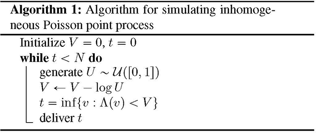
For inhomogeneous Poisson process with intensity funciton λ(t), we simulate the time interval based on a well-known algorithm. We, first define the cumulated intensity:

$$\mathrm{\Lambda }(t)={\int }_0^t\lambda (s)ds,$$

then generate the location of jumps t_j by the Algorithm 1.