A novel Ontology-guided Attribute Partitioning ensemble learning model for early prediction of cognitive deficits using quantitative Structural MRI in very preterm infants

Abstract

Structural magnetic resonance imaging studies have shown that brain anatomical abnormalities are associated with cognitive deficits in preterm infants. Brain maturation and geometric features can be used with machine learning models for predicting later neurodevelopmental deficits. However, traditional machine learning models would suffer from a large feature-to-instance ratio (i.e., a large number of features but a small number of instances/samples). Ensemble learning is a paradigm that strategically generates and integrates a library of machine learning classifiers and has been successfully used on a wide variety of predictive modeling problems to boost model performance. Attribute (i.e., feature) bagging method is the most commonly used feature partitioning scheme, which randomly and repeatedly draws feature subsets from the entire feature set. Although attribute bagging method can effectively reduce feature dimensionality to handle the large feature-to-instance ratio, it lacks consideration of domain knowledge and latent relationship among features. In this study, we proposed a novel Ontology-guided Attribute Partitioning (OAP) method to better draw feature subsets by considering the domain-specific relationship among features. With the better-partitioned feature subsets, we developed an ensemble learning framework, which is referred to as OAP-Ensemble Learning (OAP-EL). We applied the OAP-EL to predict cognitive deficits at 2 years of age using quantitative brain maturation and geometric features obtained at term equivalent age in very preterm infants. We demonstrated that the proposed OAP-EL approach significantly outperformed the peer ensemble learning and traditional machine learning approaches.

1. Introduction

The prevalence of neurodevelopmental impairments remains very high for very preterm infants (gestational age; GA ≤32 weeks), though the global infant mortality rate has been reduced to approximately 11.1% (Blencowe et al., 2013). Around 35–40% of very preterm infants develop cognitive deficits at 2 years of corrected age (Blencowe et al., 2012; Hamilton et al., 2014). Cognitive deficits would result in difficulties in academic performance and social abilities, affecting the entire life of those very preterm infants. Unfortunately, an accurate clinical diagnosis of cognitive deficits is currently unavailable for very preterm infants until 3–5 years of age in early childhood, thereby, the absence of prompt treatment leads to missing optimal neuroplasticity period of brain development when interventions can exert the greatest impact on prevention. Thus, a timely and accurate risk stratification approach is desirable to address the need for early prediction of cognitive deficits in very preterm infants.

Multiple structural magnetic resonance imaging (sMRI) studies have shown that several brain anatomical abnormalities are associated with cognitive deficits in preterm infants (Fleiss et al., 2020; Inder et al., 2005; Rathbone et al., 2011; Steinman et al., 2009). Altered cortical development has been detected on brain sMRI images in very preterm infants at term-equivalent age. For example, greater cortical thickness in frontal, insular, and anterior parietal cortices was observed in preterm infants compared with term infants (Bouyssi-Kobar et al., 2018; Kline et al., 2020; Parikh, 2016). These studies demonstrate the promise of brain maturation and geometric features as predictive biomarkers for later neurodevelopmental deficits. Recently, we developed a machine learning model to predict neurodevelopmental outcomes at 2-year corrected age using brain geometric features (e.g., volume, cortical thickness, etc.) derived from T2-weighted MRI scans collected at term-equivalent age in 110 very preterm infants (Kline et al., 2020), demonstrating the predictive abilities of those features for abnormal neurodevelopment. However, our traditional machine learning model still suffered from a large feature-to-instance ratio (i.e., a large number of features but a small number of instances/samples).

Ensemble learning is a machine learning paradigm that strategically generates and integrates a library of machine learning classifiers, referred to as base-classifiers. Unlike traditional machine learning models that only learn one hypothesis, ensemble learning defines a set of hypotheses using base-classifiers in the model library and summarizes them into a final decision. Since each base-classifier has its own strengths and weaknesses, it, therefore, is natural to expect that a learning method that takes advantage of multiple base-classifiers would lead to superior performance beyond the level obtained by any of the individual classifiers (Dong et al., 2020). In the last decade, the ensemble learning model has been successfully used on a wide variety of predictive modeling problems to boost model performance (Zhang and Ma, 2012).

Building a diverse base-classifier library is essential in any ensemble learning strategy. Attribute (i.e., feature) bagging (also known as random subspace) method (Bryll et al., 2003; Ho, 1998) is the most commonly used feature partitioning scheme, which randomly and repeatedly draws feature subsets from the entire feature set to train base-classifiers, instead of using the whole feature set. Attribute bagging method is able to effectively reduce feature dimensionality for each base-classifier and increase model diversity, offering an elegant feature partitioning solution to handle the large feature-to-instance ratio in neuroimaging studies (Kuncheva et al., 2010). However, attribute bagging through random drawing lacks consideration of domain knowledge and latent relationship among features. For example, random feature drawing simply treats the attributes of “left amygdala volume” and “right amygdala volume” as two anonymous attributes (i.e., only considers their numerical values), without noting that both quantify “volumes”; but one for “left amygdala”, and the other for “right amygdala”.

Ontology is defined as an explicit specification of a “conceptualization” or “knowledge” in a domain of interest (Grüninger and Fox, 1995; Staab et al., 2001; Uschold and Gruninger, 1996), and it has been employed for knowledge encoding, sharing, and storing (Consortium, 2004; Kulmanov et al., 2020; Smith et al., 2005). Ontology-driven techniques are increasingly being employed in a variety of biomedical research studies, such as protein-protein interactions prediction (Zhang and Tang, 2016), clinical diagnosis (Shen et al., 2018), and biological function reasoning (Köhler et al., 2009). In this study, we proposed an Ontology-guided Attribute Partitioning (OAP) method to better draw feature subsets by considering the domain-specific relationship among features, which are not considered by the standard attribute partitioning methods (e.g., attribute bagging method) (Bryll et al., 2003; Ho, 1998). With the better partitioned feature subsets, we trained and integrated a stacking/ensemble of diverse individual base-classifiers. We refer to this framework as OAP-Ensemble Learning (OAP-EL). We applied the OAP-EL to predict cognitive deficits at 2 years of age using quantitative brain maturation and geometric features obtained at term-equivalent age in very preterm infants. We tested the hypothesis that the proposed OAP-EL approach can significantly outperform the peer ensemble learning approaches with attribute bagging method.

2. Materials and methods

2.1. Overview

Our clinical task in this study is to stratify the risk of cognitive deficits in very preterm infants at 2 years corrected age based on quantitative brain maturation and geometric features acquired on structural MRI at term-equivalent age. As shown in Fig. 1, we first extract hundreds of brain maturation and geometric features from T2-weighted MRI data acquired at term-equivalent age for individual very preterm infants using the Developing Human Connectome Project (dHCP) processing pipeline (Makropoulos et al., 2018) (Fig. 1A). Next, based on two prior defined ontologies, which respectively describe brain parcellation (e.g., frontal lobe, temporal lobe, parietal lobe, etc.) (Gousias et al., 2012), and brain geometry and maturation (cortical thickness, sulcal depth, curvature, cortical surface area, etc.) (Makropoulos et al., 2018), we construct an unweighted ontology graph, in which brain maturation and geometric features are considered as vertices and ontology-derived relationships are edges. We then conduct ontology graph clustering (Fig. 1B) to partition brain maturation and geometric features into k non-overlapping feature subsets (Fig. 1C). With k feature subsets, we train k base-classifiers (i.e., eXtreme Gradient Boosting (XGBoost) classifiers (Chen and Guestrin 2016)) in this work. Finally, a neural network is used as the meta-classifier to integrate k individual base-classifiers for risk stratification (Fig. 1D).

Fig. 1.

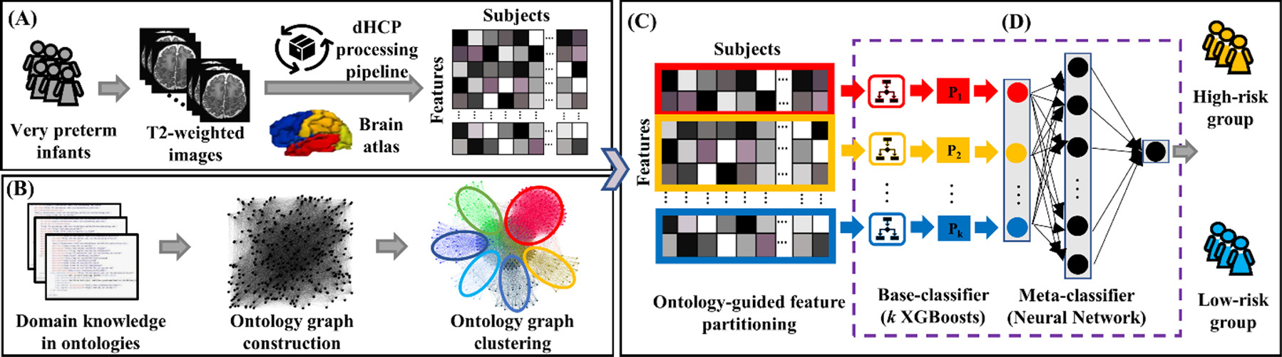
Schematic diagram of OAP-EL for early prediction of cognitive deficits at 2 years corrected age using brain maturation and geometric features derived from T2-weighted MRI acquired at term-equivalent age in very preterm infants. (A) Brain maturation and geometric feature extraction; (B) Ontology graph construction and clustering; (C) Ontology-guided feature partitioning; and (D) Base-classifiers training and ensembling.

2.2. MRI data acquisition and follow-up cognitive assessment

The cohort from the CCHMC site consisted of very preterm infants from the Cincinnati Infant Neurodevelopment Early Prediction Study (referred to as CINEPS Cohort) (Parikh et al., 2021). All infants born at or before 32 weeks of GA, between September 2016 and November 2019, who were cared for in one of the five level III/IV Cincinnati, Ohio Neonatal Intensive Care Units (NICUs), including CCHMC, University of Cincinnati Medical Center, Good Samaritan Hospital, St. Elizabeth’s Healthcare, and Kettering Memorial Hospital, were eligible for CINEPS inclusion. The other cohort from the NCH site (referred to as the Columbus Early Prediction Study [COEPS]) enrolled very preterm infants born at 31 weeks GA or younger (between December 2014 and April 2016) from one of the four level III/IV Columbus, Ohio NICUs, including NCH, Ohio State University Medical Center, Riverside Hospital, and Mount Carmel St. Ann’s Hospital. After initial recruitment discussion and related consent, all very preterm infants were medically transported to either the CCHMC site (CINEPS cohort) or the NCH site (COEPS cohort) for their MRI scans after NICU discharge. Infants were excluded from both CINEPS and COEPS cohort, if any known congenital brain anomalies or severe injury was observed (Logan et al., 2021). The CINEPS cohort was used for model development and internal cross validation, while the independent COEPS cohort was used as an unseen testing dataset for external validation.

At CCHMC site, CINEPS subjects were imaged at 39–44 weeks postmenstrual age (PMA) during unsedated sleep on a 3T Philips Ingenia scanner with a 32-channel receiver head coil. Acquisition parameters for axial T2-weighted turbo spin-echo sequence are repetition time (TR) = 8300 ms, echo time (TE) = 166 ms, FA = 90°, resolution 1.0 × 1.0 × 1.0 mm³, and time 3:53 min. At NCH site, COEPS subjects were scanned at 38–43 weeks PMA during unsedated sleep on a 3T MRI scanner (Skyra; Siemens Healthcare) using a 32-channel receiver head coil. Acquisition parameters for axial T2-weighted fast spin-echo sequence are TR = 9500 ms, TE = 147 ms, FA = 150°, resolution 0.93 × 0.93 × 1.0 mm³, and time 4:09 min.

All subjects were assessed at 2 years of corrected age using the well-established Bayley Scales of Infant and Toddler Development III (Bayley III) test (Bayley, 2006). The Bayley III Cognitive subtest scores (on a scale of 40 –160, with a mean of 100 and a standard deviation shown (SD) of 15) served as the primary measures of the infant’s cognitive development functioning level.

2.3. MRI data preprocessing and brain maturation and geometric feature extraction

We preprocessed T2-weighted MRI data of each subject and extracted brain maturation and geometric features using dHCP structural pipeline (Makropoulos et al., 2018). Briefly, the pipeline conducted bias field correction (Tustison et al., 2010), brain extraction (Smith, 2002; Makropoulos et al., 2014), and brain surface reconstruction (Schuh et al., 2017). The pipeline segmented the whole brain image into 87 region-of-interests (ROIs) based on an age-matched neonatal volumetric atlas (Gousias et al., 2012; Smith, 2002). For individual brain ROIs, up to six different types of brain maturation and geometric metrics were calculated, including volume, thickness, sulcal depth, curvature, gyrification index, and surface area. It is worth noting that, for some ROIs, not all aforementioned metrics are available. For example, dHCP pipeline only extracts the volume metric for the hippocampus. In addition, dHCP pipeline calculates both absolute and relative measures for volume and surface area metrics, which are highly dependent on individual brain sizes. The relative measures are calculated using the absolute measures divided by whole-brain measures. A total of 510 brain maturation and geometric features were calculated by the dHCP pipeline from the whole brain. For both volume and surface area metric types, we only retained relative measures to reduce the impact of individual brain size variance. In this way, we obtained a list of 338 brain maturation and geometric features from individual T2-weighted MRI data for our subjects. We provided the full list of 510 features and the final list of 338 features in the Supplemental Materials. This brain feature vector (1 × 338) was utilized as input of our proposed OAP-EL model. Meanwhile, an ontology graph can be constructed (Section 2.4), in which the number of nodes within the graph is equal to the number of features (i.e., 338 features).

2.4. Ontology graph construction

We designated latent relationship among features through building an ontology graph by utilizing two prior-defined ontologies that respectively define brain parcellation as well as brain maturation and geometry. The brain parcellation ontology describes the whole brain segmented into 9 tissues (e.g., cortical grey matter, white matter, and etc.) (Makropoulos et al., 2018), and 87 regions (Makropoulos et al., 2018; Gousias et al., 2012; Makropoulos et al., 2014) (e.g., Frontal lobe, Hippocampus, Corpus, Insula, etc.). The brain maturation and geometry ontology lists six brain maturation metrics, including volumes, cortical thickness, sulcal depth, curvature, gyrification index, and surface area (Makropoulos et al., 2018). To facilitate knowledge sharing, we expressed these two ontologies in the Web Ontology Language (OWL) format, which can be read or visualized by typical OWL processing packages, such as Owlready2 in Python (Data and Code Availability).

Utilizing domain knowledge stored in the above-mentioned two ontologies, we constructed an unweighted ontology graph G, in which dHCP brain maturation and geometric features (i.e., 338 features from dHCP pipeline) were considered as vertices V = [v_1, …, v_n], and ontology-derived relationships were edges E = [e₁, …, e_n]. The value of the edge e_ij ∈ E between two vertices v_i and v_j ∀i, j ∈ n was set to be 1, if two features quantify the same brain maturation and geometric metrics (e.g., the volume of left frontal lobe and the volume of left occipital lobe) or describe the same brain parcellations (e.g., the volume of left occipital lobe and the surface area of left occipital lobe), otherwise, we set it to 0 (Fig. 2).

Fig. 2.

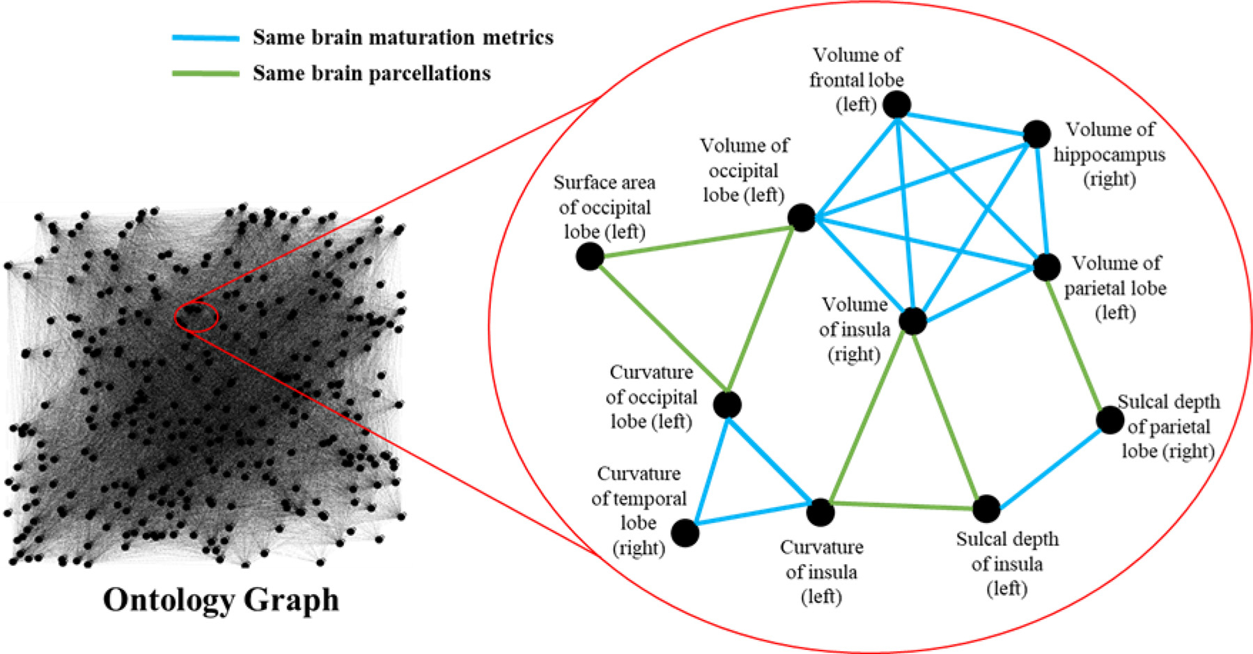
Ontology graph with an enlarged subgraph. Based on domain knowledge within two pre-defined ontologies, two vertices are connected if they quantified the same brain maturation and geometric metrics or describe the same brain parcellations, otherwise they are disconnected.

2.5. Ontology-guided Attribute Partitioning ensemble learning (OAP-EL) model

In contrast to the most commonly used attribute bagging method (Bryll et al., 2003; Ho, 1998), we conducted ontology graph clustering via a spectral clustering algorithm (Shi and Malik, 2000) for feature partitioning. Given our unweighted ontology graph G = (V, E), the graph Laplacian matrix is defined as L = D – A, where similarity matrix A of the graph G, and D is a degree matrix of graph G. Since L ∈ R^n×n is a positive semidefinite matrix, the eigendecomposition of L is defined as L = U ΛU⁻¹, where U ∈ R^n×n, whose i_th column is the eigenvector u_i of U, and $\mathrm{\Lambda }\in Z_{\ge 0}^{n\times n}$ is a diagonal matrix whose diagonal elements Λ_ii = λ_i corresponding to its eigenvalue. The spectral clustering algorithm outputs k sets of cluster labels by performing a k-means on the first k eigenvectors U_k of L, such that, U_k ∈ R^n×k ⊆ U. The number of clusters k is a hyperparameter that can be optimized based on the performance of downstream tasks. We finally partitioned brain maturation and geometric features into k non-overlapping feature subsets.

Using k non-overlapped OAP feature subsets, we built k XGBoost models (Chen and Guestrin, 2016) as base-classifiers. Assume that c_i ∈ C ∀i ∈ [1, …, k] is the i_th OAP feature subset, and $f_i^b\in F^b\forall i\in [1,\dots ,k]$ represents i_th base-classifier. To train each $f_i^b$, we minimized the loss function:

$$L(\varphi )=\sum _{i=1}^{N}l\left(y_i,{\widehat{y}}_i\right)+\gamma T+\sum _{j=1}^T\frac{1}{2}\eta s_j^2$$ (2)

where $l\left(y_i,{\widehat{y}}_i\right)$ represents the convex function between true label y_i and prediction ${\widehat{y}}_i$, γ and η represent the shrinkage parameters for penalizing the model complexity through adjusting the number of leave node j which corresponds to its output of scores s_j. Each $f_i^b$ takes the input of a dataset corresponding to a c_i and produces a probabilistic outcome ${\widehat{p}}_i=f_i^b\left(c_i\right)\forall i\in [1,\dots ,\text{k}]$. Hence, $\widehat{P}=F^b(C)$ where $\widehat{P}=\left[{\widehat{p}}_1,\dots ,{\widehat{p}}_{\text{k}}\right]$ represents a set of probabilities from F^b that will be the input for the metaclassifiers.

We used a neural network model as meta-classifier f^m to integrate k probabilities ${\widehat{p}}_i\in \widehat{P}\forall i\in [1,\dots ,k]$ of $f_i^b\in F^b\forall i\in [1,\dots ,k]$. The neural network contains an input layer, a fully connected hidden layer with a Rectified Linear Unit (ReLU) as activation function, and an output layer using a sigmoid function. The final probabilistic outcome ${\widehat{p}}^{*}$ can be defined as ${\widehat{p}}^{*}=f^m(\widehat{P})={[1+\exp (-{(0,W\widehat{P}+b)}^{+})]}^{-1}$, where W and b are the weight matrix and bias. To train f^m, we minimized the binary cross entropy loss function with L₂ norm regularization, which was given by

$${ℒ}^{*}=-\frac{1}{M}\sum _{i=1}^M\left[y_i\log {\widehat{p}}^{*}+\left(1-y_i\right)\log \left(1-{\widehat{p}}^{*}\right)\right]+\lambda \Vert W{\Vert }^2$$ (3)

where M is the sample size, y_i represents the i_th class label ∀i ∈ [1, …, M], and λ is the coefficient of L₂ norm regularization, penalizing the weight matrix W to avoid the overfitting problem. For selecting the hyperparameters of λ and maximum depth m, we tuned the model using a grid search (i.e., λ = [0.001, 0.01, 0.1]; m =[2, 4, 6, 8]). We trained the neural network for the meta-classifiers with 1000 epochs using an Adam optimization algorithm with a learning rate of 0.01, and λ = 0.001 was chosen for L₂ norm regularization.

2.6. Internal and external model validation

We evaluated the proposed OAP-EL model using both internal and external validation experiments with performance metrics of accuracy, sensitivity, specificity, and area under the receiver operating characteristic (ROC) curve (AUC). To evaluate the model performance on positive minority samples, we plotted Precision-Recall (PR) curves and calculated area under the PR curve (PRAUC). We further reported the mean and standard deviation of performance metrics from 100 experiment replications. For internal validation, we trained and tested the model using CINEPS cohort with a nested Leave-One-Out Cross Validation (LOOCV) strategy, which includes an outer loop and an inner loop. In the outer LOOCV loop, we separated the dataset into training-validation data (N-1 samples) and testing data (1 sample) in each of N iterations and repeated this process iteratively until all subjects were treated as testing data. Performance metrics were calculated on testing data. In the inner LOOCV loop, the model hyperparameters were optimized using training-validation data (N-1 samples) without seeing any testing data. For external validation, we tested the internally validated model using the unseen independent COEPS cohort.

To handle the data imbalance issue, we applied a data synthesis approach on the training dataset after LOOCV data split. For the CINEPS dataset, we have a smaller number of very preterm infants in the high-risk group compared to those in the low-risk group with a ratio of 1:2. With an imbalanced dataset, machine learning models are prone to become majority class classifiers, i.e., they fail to learn the concepts of the minority class. To overcome this challenge, we first generated new synthetic samples for minority class (for model training only) using synthetic minority over-sampling (SMOTE) method (Chawla et al., 2002). Specifically, we randomly selected a sample from the minority class and obtained its five nearest neighbors. We interpolated new synthetic samples between the selected minor sample and its nearest neighbors. We repeated this process until the ratio of high-risk and low-risk subjects in the training dataset was 1:1. Next, we implemented edited nearest neighbor (ENN) method (Batista et al., 2004). We also selected a random sample in the majority class and obtained its five nearest neighbors. If the class of selected sample was different from its five nearest neighbors, these samples were removed regardless their class labels in majority or minority class. This process was repeated until the ratio of high-risk and low-risk subjects in the training dataset was 1:1. The procedure was referred to as SMOTE-ENN method (Batista et al., 2004) with additional details illustrated in the Supplementary Table 1.

We compared our proposed model with (1) traditional machine learning models, including K-Nearest Neighbor (KNN) (Fix and Hodges, 1989), Logistic Regression (LR) (Cox, 1958), Support Vector Machine (SVM) (Cortes and Vapnik, 1995), Decision Tree (DT) (Wu et al., 2008), Random Forest (RF) (Ho, 1995), Neural Network (NN) (McCulloch and Pitts, 1943); (2) peer ensemble learning models, including Voting (Dietterich, 2002), Bagging (Breiman, 1996), Stacking (Wolpert, 1992), and Attribute Bagging-Ensemble Learning (AB-EL); and (3) Multi-Channel Neural Networks (mNN) that was developed in our prior study (Chen et al., 2019). The detailed implementation of all the models can be found in Supplemental Materials. All the machine learning experiments were performed in a workstation with a processor with Intel(R) Core(TM) i5–10600KF CPU at 4.10 GHz, 8 GB RAM, and a NVIDIA GeForce GTX 1660 SUPER GPU. Experiment coding was conducted using Python 3.7, TensorFlow 2.3.0, and Scikit-Learn 0.24.1.

2.7. Identification of discriminative features

We identified and reported the top discriminative brain geometric features that contributed most to the prediction of cognitive deficit by utilizing a two-level feature importance ranking strategy. Within our OAP-EL model, suppose that W represents the connection weights of the meta-classifier, and weight w_i ∈ W ∀i ∈ [1, …, k] corresponds to the i_th base-classifier. Let β_ij ∈ B_i ∀j ∈ [1, .., |c_i|], c_i ∈ C be the j_th feature importance score of i_th XGBoost base-classifier using the information gain (Azhagusundari and Thanamani, 2013), where |c_i| is the size of features within the i_th base-classifier. The global ranking score of a brain maturation and geometric feature is defined as $\frac{w_i}{{\sum }_{i=1}^k{w}_i}\cdot \frac{{\beta }_{ij}}{max\left({\text{B}}_i\right)}$.

2.8. Statistical analysis

To examine demographic differences between the groups of high-risk and low-risk infants, we used two-sample Student’s t-test to compare means for continuous variables, including birth weight, gestational age (GA) at birth, postmenstrual age (PMA) at scan and cognitive score, and Pearson’s chi-squared test to compare gender distribution. To compare the different prognostic models, we used the nonparametric Wilcoxon test. A p-value less than 0.05 was considered statistically significant for all inference testing. All statistical analyses were conducted in R-4.0.3 (RStudio, Boston, MA, USA).

3. Results

3.1. Finding the optimal number of feature clusters k

The number of feature clusters was optimized using the internal validation cohort. Specifically, we tested the numbers of clusters k with empirical values from 1 to 100 in increments of 1. For each k, we repeated nested LOOCV 100 times to evaluate prediction performance. Fig. 3(A) shows the mean AUC with various numbers of clusters k. According to the highest mean AUC, we set the optimal number of feature clusters to be 6 in the following experiments. Further, we applied silhouette score to evaluate the goodness of ontology-guided clustering. Silhouette score is a measure of how similar an object (i.e., feature) is to its own cluster compared to other clusters. It ranges from −1 to +1, where a higher value indicates that objects are clustered better. We calculated a silhouette score for each feature in our ontology graph, and then averaged silhouette scores across all features. A detailed calculation of the mean silhouette score is included in the Supplemental Material. Fig. 3(B) shows that the optimal number of feature clusters (k = 6) appears to have the highest silhouette score compared to the other numbers of feature clusters, demonstrating that our proposed OAP is able to partition features into better clusters by only using prior domain knowledge. Besides, the ontology graph (k = 6) using spectral clustering is shown in Fig. 4. The bubbles and link represent the sample nodes (i.e., features) and edges to illustrate some clustered feature examples.

Fig. 3.

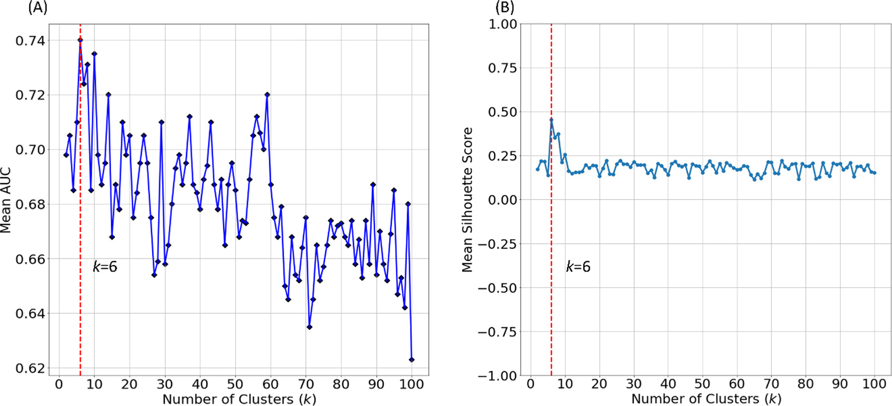
Optimization of the number of feature clusters k for early prediction of cognitive deficits in very preterm infants. (A) mean AUC of the predictive model with varying numbers of clusters. (B) mean silhouette scores of varying numbers of clusters.

Fig. 4.

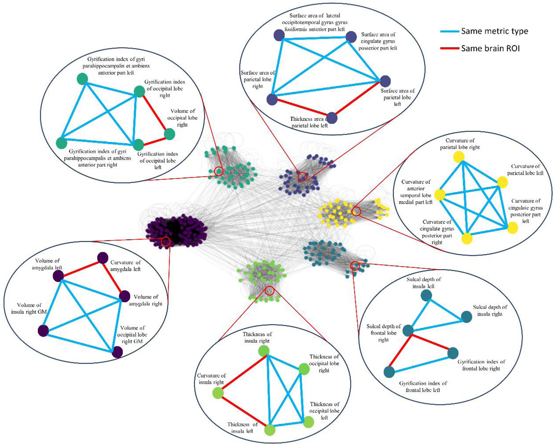
Ontology graph partitioned using spectral clustering algorithm into the optimal number of clusters (k = 6). Sample nodes and edges in each cluster are displayed in the bubble. Nodes are colored according to their clusters. Edge colors are added in indicate same metric type (blue) or same brain ROI (red).

We further analyzed the feature clusters derived from our OAP approach. We illustrated the distribution of the feature types and representative ROIs in each one of six feature clusters. (Fig. 5) We noted from Fig. 5(A) that each feature cluster generated from the ontology graph is dominated by one feature type, and none of feature cluster contains a single feature type. This clearly demonstrates that different types of brain metrics have complementary information, which may improve the discriminative power of base-classifiers. On the other hand, from Fig. 5(B), we observed that all feature clusters were dominated by features related to temporal lobe. This is simply because that the adopted brain parcellation ontology divided the temporal lobe into more subregions than other major brain lobes and regions, resulting more features from temporal lobe.

Fig. 5.

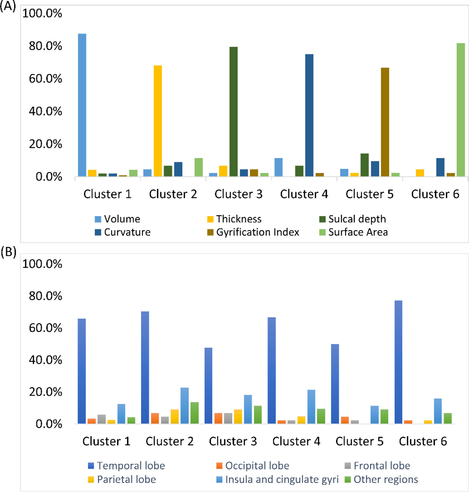
The distribution of (A) brain metrics and (B) brain regions among feature clusters. For those brain regions (hippocampus, amygdala, cerebellum, cerebrospinal fluid) that contain very few features, we merged them together as ‘other regions’ for visualization purpose.

3.2. Internal validation with CINEPS cohort

We included 207 very preterm infants (mean (SD) GA of 29.4 (2.4) weeks; birth weight of 1288.3 (434.5) g) who completed 2-year cognitive assessments from CINEPS cohort for internal validation. (Table 1) We defined infants with a Bayley III cognitive score less than or equal to 85 (i.e., 1 SD below the mean score) as the high-risk group (N = 69) and those with a cognitive score greater than 85 as the low-risk group (N = 138) for developing cognitive deficits. The sample ratio between the high- and low-risk groups was 1:2 in the CINEPS cohort. The high-risk group had a mean GA of 28.7 (2.7) weeks, PMA of 42.5 (1.3) weeks, birth weight of 1184.1 (489.3) g, and 43 of 69 (62.3%) subjects were male. The low-risk group had a mean GA of 29.7 (2.2) weeks, PMA of 42.4 (1.3) weeks, birth weight of 1340.5 (397.3) g, and 67 of 138 (48.6%) subjects were male. Between groups, there was significant difference in birth weight (p = 0.02), gestational age at birth (p < 0.001) and cognitive scores (p < 0.001); and no significant difference in sex (p = 0.08) and postmenstrual age at scan (p = 0.48).

Table 1.

Demographics summary of CINEPS cohort.

	CINES Cohort Low-risk (N = 138)	High-risk (N = 69)	p-value
Male sex; Number (%)	67 (48.6%)	43 (62.3%)	0.08
PMA at scan in weeks; Mean (SD)	42.4 (1.3)	42.5 (1.3)	0.48
GA in weeks; Mean (SD)	29.7 (2.2)	28.7 (2.7)	< 0.001
Birth weight in grams; Mean (SD)	1340.5 (397.3)	1184.1 (487.3)	0.02
Cognitive assessment at 2 years corrected age; Mean (SD)	99.2 (8.8)	76.0 (10.7)	< 0.001

3.2.1. Effects of individual ontologies on OAP-EL

We first investigated the effects of individual ontologies on our early prediction task. We constructed three ontology graphs using (1) brain metric ontology, (2) brain parcellation ontology, and (3) combined ontologies, respectively. Feature clustering was performed on all ontology graphs, and OAP-EL models were developed using the internal cohort. As shown in Table 2, the OAP-EL model using combined ontologies achieved a mean AUC of 0.74, significantly higher than the OAP-EL models using either brain metric ontology (AUC = 0.69, p < 0.001) or brain parcellation ontology (AUC = 0.61, p < 0.001). This demonstrates that individual brain ontologies have their own discriminative power, and combining ontologies together is able to further increase the overall discriminative power by using complementary knowledge from individual ontologies.

Table 2.

Model performance of the proposed OAP-EL using brain metric ontology, brain parcellation ontology, and combined ontologies.

Ontologies	Accuracy (%)	Sensitivity (%)	Specificity (%)	AUC
Brain metric ontology	69.1 (3.1)	67.3 (3.8)	70.3 (2.9)	0.69 (0.03)
Brain parcellation ontology	61.7 (3.4)	61.9 (4.2)	63.5 (3.2)	0.61 (0.04)
Combined ontologies	71.3 (1.9)	70.6 (2.0)	72.6 (1.7)	0.74 (0.03)

3.2.2. OAP-EL outperforms traditional machine learning models

Fig. 6 shows the performance comparison among our proposed OAP-EL model and traditional machine learning models in the detection of very preterm infants at high risk for moderate/severe cognitive deficits. Compared to the best performing traditional machine learning model, SVM, our proposed OAP-EL model significantly improved accuracy by 8.2% (p < 0.001), sensitivity by 9.0% (p < 0.001), specificity by 7.5% < 0.001), and AUC by 0.1 (p < 0.001).

Fig. 6.

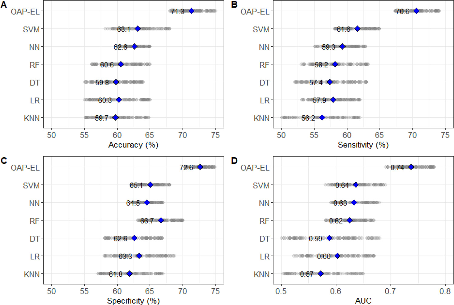
Internal validation of the proposed OAP-EL and traditional machine learning models on (A) Accuracy, (B) Sensitivity, (C) Specificity, and (D) AUC. KNN: K-nearest neighbor; LR: Logistic Regression; SVM: Support Vector Machine; DT: Decision Tree; RF: Random Forest; NN: Neural Network; OAP-EL: Ontology-guided Attribute Partitioning Ensemble Learning. The highlight points indicate the mean value of measures.

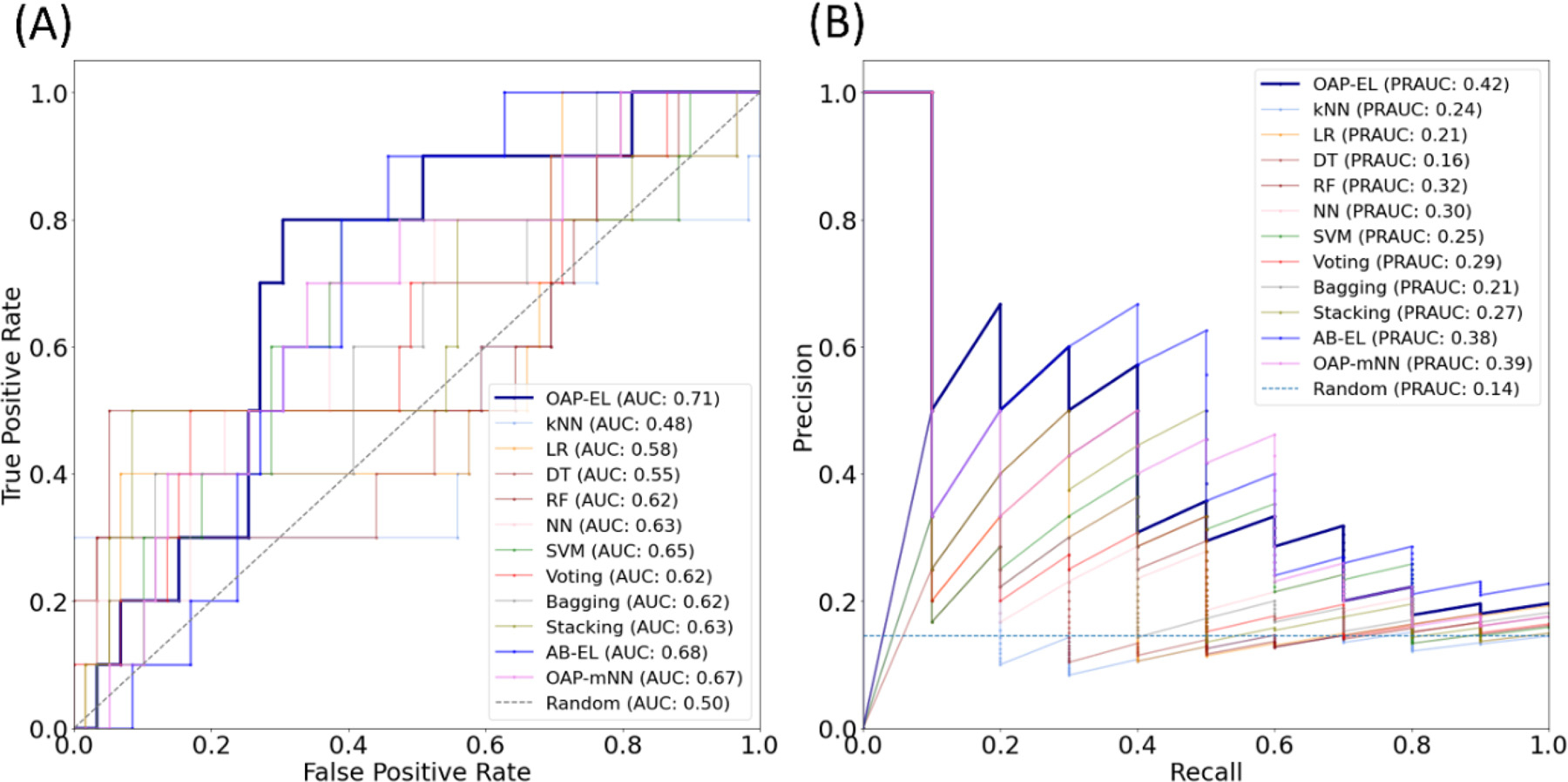
Both ROC and PR curves demonstrate that our OAP-EL model had a superior prediction performance. (Fig. 7) Our proposed OAP-EL achieved better AUC and PRAUC than other traditional machine learning models.

Fig. 7.

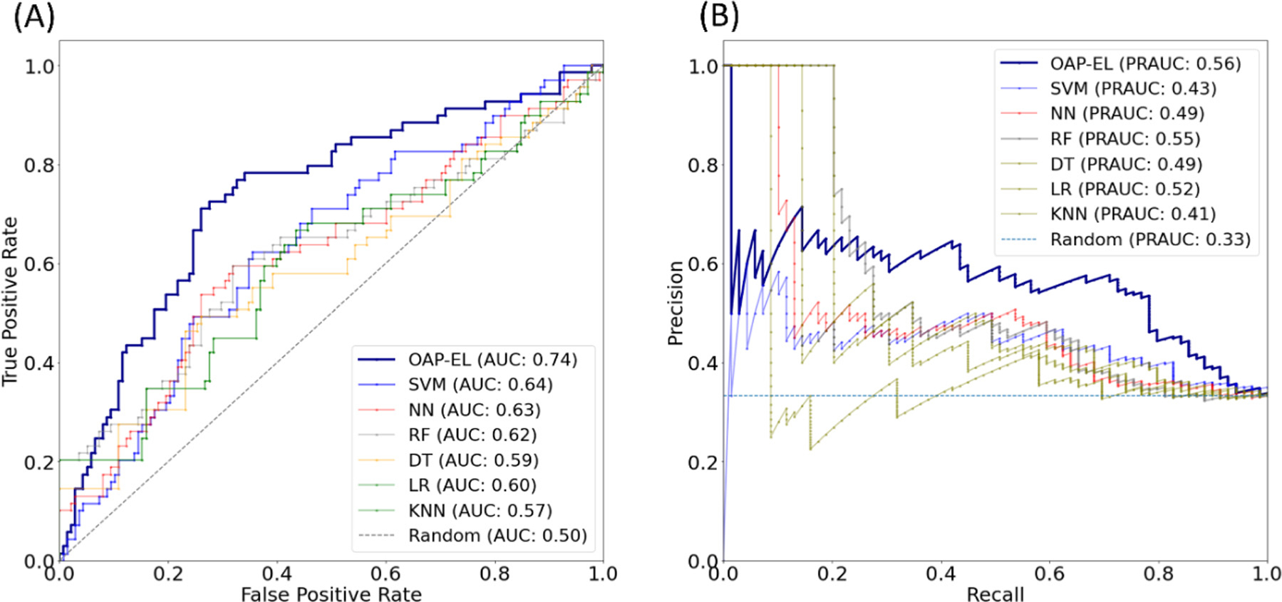
Model performance comparison between the OAP-EL method and traditional machine learning methods for internal validation using (A) receiver operating characteristic curves, and (B) precision-recall curves. AUC-Area under the ROC curve; PRAUC-Area under the Precision-Recall curve.3.2.3 OAP-EL Outperforms Peer Ensemble Learning Models

We compared the proposed OAP-EL model with several peer ensemble learning models, including Voting, Bagging, and Stacking without/with attribute bagging method. The prediction performance is shown in Table 3. Our proposed OAP-EL model achieved the best prediction performance among peer ensemble learning models. The proposed model significantly improved the prediction performance over the AB-EL model by 3.8% in accuracy (p < 0.001), 5.4% in sensitivity (p < 0.001), 4.2% in specificity, and 0.05 in AUC (p < 0.001). Fig. 8 illustrates both ROC and PR curves of ensemble learning models. While ROC curves shows that our OAP-EL model had a better prediction performance, PR curves demonstrate the superior performance of our OAP-EL model over peer ensemble learning models with a larger margin.

Table 3.

Internal validation of the proposed OAP-EL and ensemble learning models on Accuracy, Sensitivity, Specificity, and AUC.

Model	Accuracy (%)	Sensitivity (%)	Specificity (%)	AUC
Voting	62.3 (2.5)	57.5 (2.8)	64.7 (2.3)	0.62 (0.02)
Bagging	63.4 (3.1)	62.5 (3.1)	67.1 (2.6)	0.63 (0.03)
Stacking	63.8 (4.2)	61.6 (2.1)	67.3 (2.7)	0.63 (0.03)
AB-EL	67.5 (3.8)	65.2 (4.4)	68.4 (3.5)	0.69 (0.03)
OAP-EL	71.3 (1.9)	70.6 (2.0)	72.6 (1.7)	0.74 (0.03)

AB- EL: Attribute Bagging Ensemble Learning, OAP-EL: Ontology-guided Attribute Partitioning Ensemble Learning. Experiment results are represented as mean (SD).

Fig. 8.

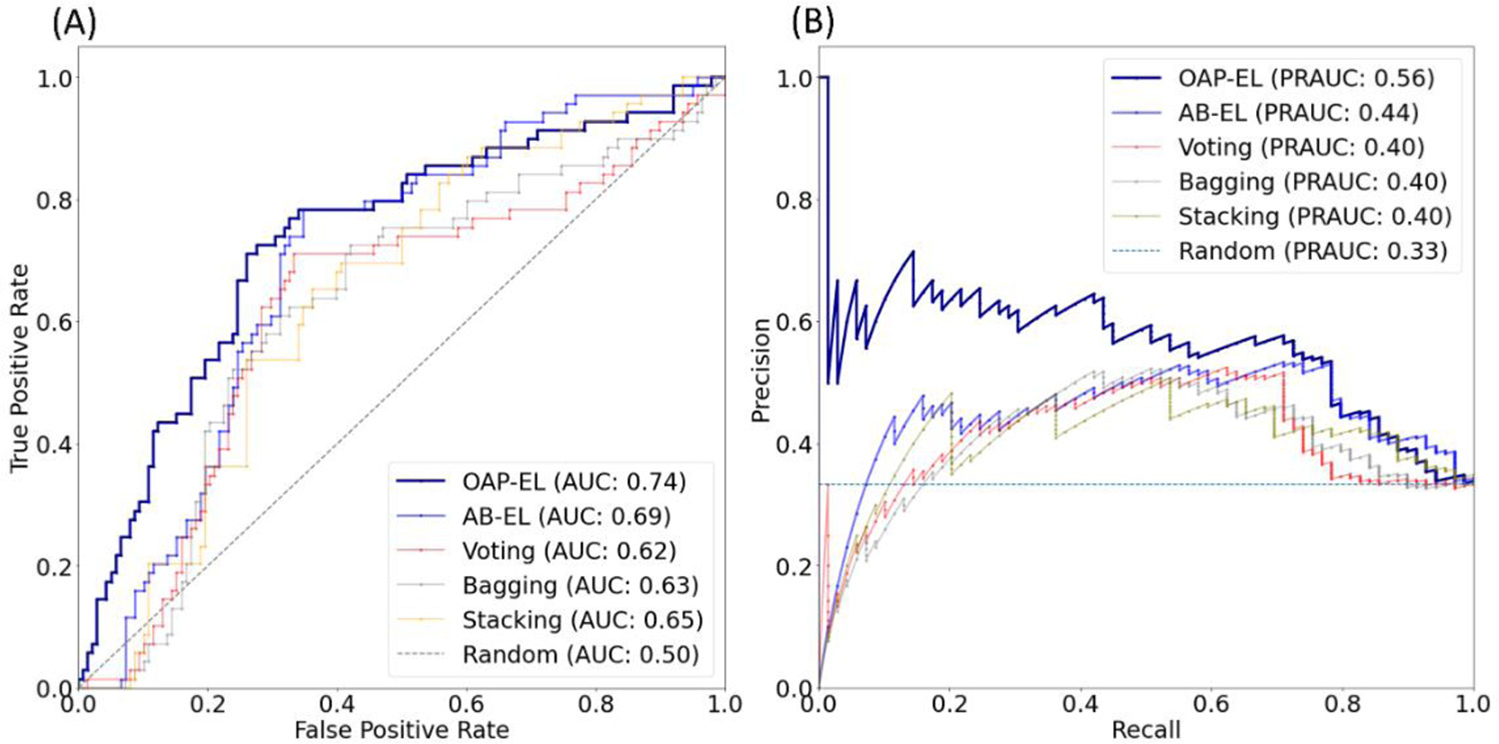
Model performance comparison between the OAP-EL method and peer ensemble learning methods for internal validation using (A) receiver operating characteristic curves, and (B) Precision-Recall curves. AUC-Area under the ROC curve; PRAUC-Area under the Precision-Recall curve.

To evaluate the effect of spectral clustering algorithm on the ontology graph, we further compared the model performance using OAP-derived feature clusters (k = 6) and random feature clusters (k = 6) (Fig. 9). The model using OAP-derived feature clusters (k = 6) achieved 71.3% accuracy, 70.6% sensitivity, 72.6% specificity, and 0.74 AUC. It was significantly better than the model using random feature clusters (k = 6) that achieved an accuracy of 64.1% (p < 0.001), sensitivity of 63.6% (p < 0.001), specificity of 67.2% (p < 0.001), and AUC of 0.66 (p < 0.001).

Fig. 9.

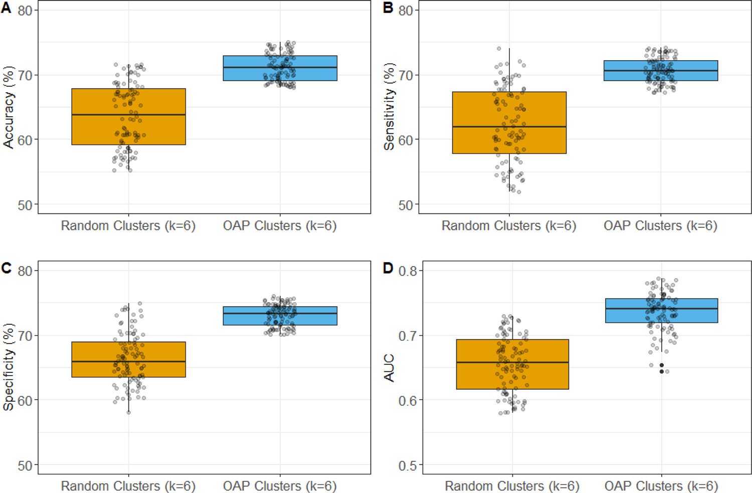
Prediction performance comparison of models using OAP-derived feature clusters (k = 6) and random feature clusters (k = 6).

3.2.4. OAP-EL outperforms OAP-enhanced Multi-Channel Neural Network (OAP-mNN)

We compared the proposed OAP-EL model with OAP-mNN model (Supplemental Materials). We observed that the proposed OAP-EL achieved significantly better prediction performance than the OAP-mNN with a margin of 5.4% (p < 0.001) in accuracy, 4.8% (p < 0.001) in sensitivity, 2.2% (p < 0.001) in specificity, and 0.04 (p < 0.001) in AUC (Fig. 10). The PR curves in Fig. 11 demonstrates that our OAP-EL model had a significantly better prediction performance than the OAP-mNN model, even though ROC curves of both OAP-EL and OAP-mNN appear comparable.

Fig. 10.

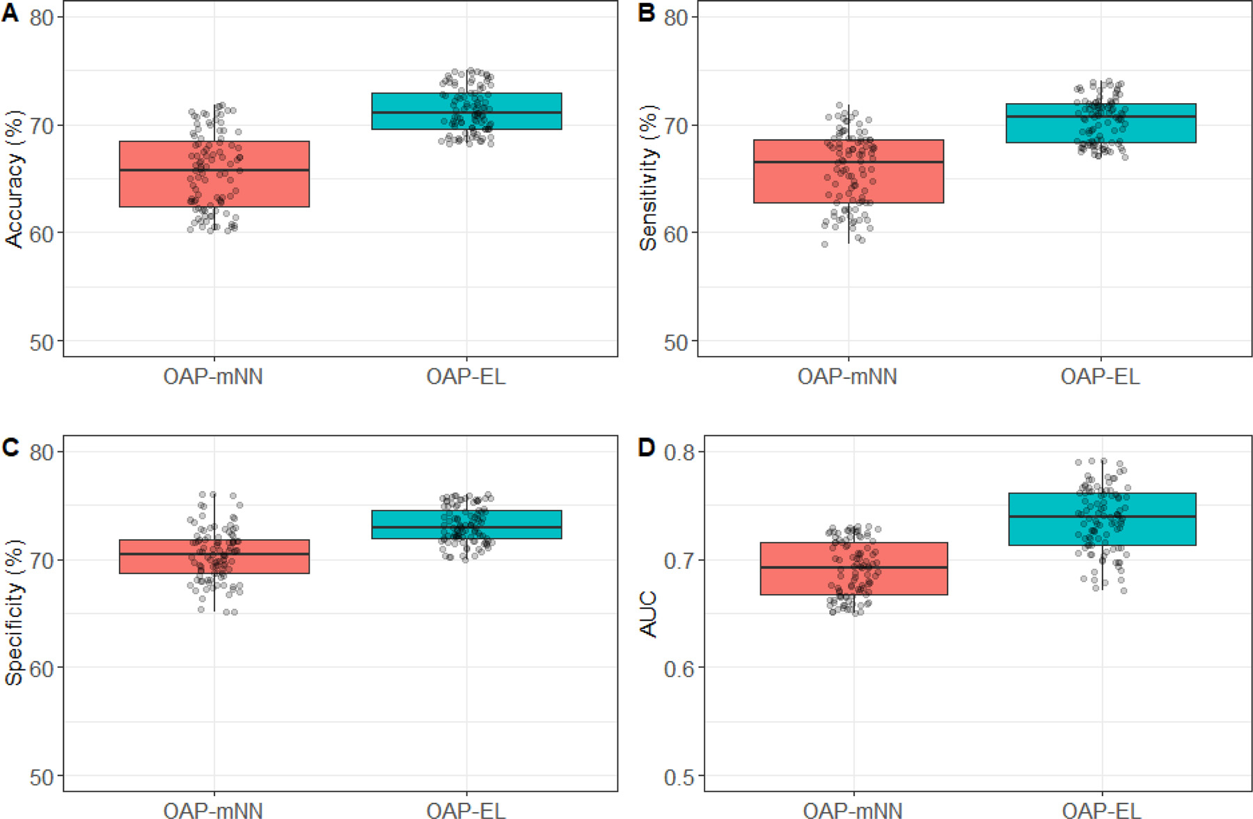
Internal risk prediction performance of cognitive deficits comparison with Multi-Channel Neural Network models on (A) Accuracy, (B) Sensitivity, (C) Specificity, and (D) AUC. OAP-mNN: Ontology-guided Attribute Partitioning Multi-Channel Neural Network; OAP-EL: Ontology-guided Attribute Partitioning Ensemble Learning.

Fig. 11.

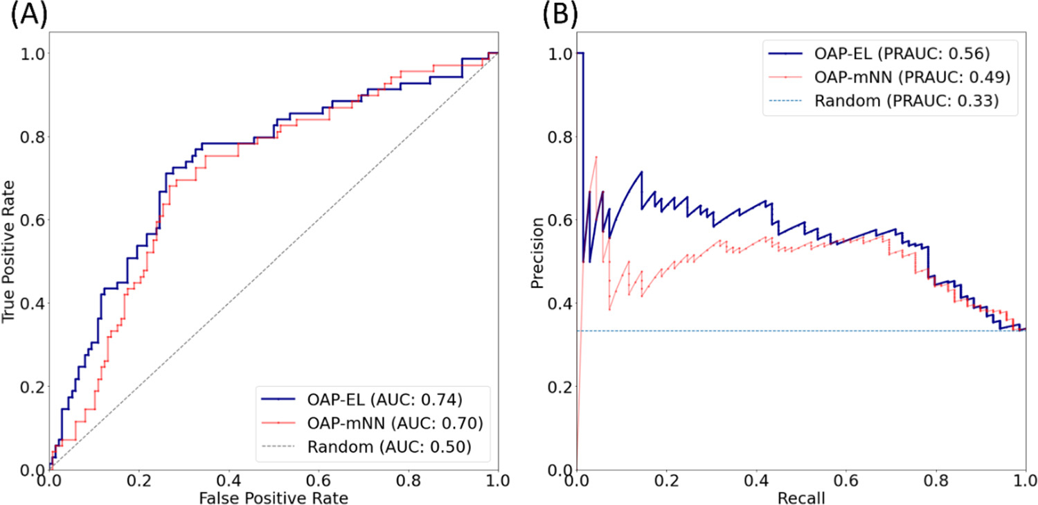
Model performance comparison between the OAP-EL method and Multi-Channel Neural Networks for internal validation using (A) receiver operating characteristic (ROC) curves, and (B) Precision-Recall curves. AUC-Area under the ROC curve; PRAUC-Area under the Precision-Recall curve.

3.2.5. An ablation study on the impact of individual brain metric types

In this section, we conducted an ablation study to assess the impact of individual brain maturation and geometry metric types. Specifically, we removed one type of metric and only utilized the rest of five types to develop and evaluate the proposed OAP-EL model. For example, we excluded all brain volume metric-related features and retained all other features in one trial. We performed a total of six trials, in each of which we excluded only one type of metric. Table 4 shows the prediction performance of OAP-EL models across all trials. The OAP-EL model achieved the best accuracy in Trial 2, where we removed all features related to the gyrification index. This indicates that the impact of gyrification index is the least among all six metric types. On the other hand, in Trial 4, where all curvature features were excluded, the OAP-EL model had the lowest mean prediction accuracy of 66.5%, compared to a mean accuracy of 71.3% when all features were included. This means that curvature features might have the largest impact on model accuracy. Overall, we observed that all six metric types have their own discriminative power on early prediction of cognitive deficits in very preterm infants.

Table 4.

An ablation study to assess the impact of individual metric types (m1-m6) on prediction performance for cognitive deficits. In each trial, one metric type was excluded and the rest of five types were utilized to develop and evaluate the proposed OAP-EL model.

Trial # No.	Metric Types						Accuracy (%)	Sensitivity (%)	Specificity (%)	AUC
	m1	m2	m3	m4	m5	m6
1	✗	✓	✓	✓	✓	✓	66.7 (2.9)	65.1 (3.6)	68.4 (3.0)	0.68 (0.02)
2	✓	✗	✓	✓	✓	✓	69.4 (3.4)	68.5 (3.5)	70.5 (3.1)	0.72 (0.03)
3	✓	✓	✗	✓	✓	✓	67.2 (4.2)	64.7 (4.1)	67.2 (2.4)	0.65 (0.03)
4	✓	✓	✓	✗	✓	✓	66.5 (3.6)	65.9 (4.5)	66.4 (3.3)	0.67 (0.04)
5	✓	✓	✓	✓	✗	✓	68.5 (3.1)	67.4 (3.8)	69.3 (2.8)	0.70 (0.02)
6	✓	✓	✓	✓	✓	✗	66.8 (3.9)	64.0 (4.7)	68.1 (3.9)	0.65 (0.03)
All	✓	✓	✓	✓	✓	✓	71.3 (1.9)	70.6 (2.0)	72.6 (1.7)	0.74 (0.03)

m₁ : volume; m₂ : gyrification index; m₃ : thickness; m₄ : curvature; m₅ : surface area; m₆ : sulcal depth

3.3. External validation with COEPS cohort

We included 69 very preterm infants with mean (SD) GA of 28.2 (2.4) and birth weight of 1123.6 (400.1) from the independent COEPS cohort for external validation. (Table 5) Like the CINEPS cohort, we used a Bayley III 85 as the cutoff score to stratify the risk of cognitive deficits. Infants with a score less than or equal to 85 were defined as a high-risk group (N = 10), while infants with a score greater than 85 were defined as a low-risk group (N = 59). The sample ratio between high- and low-risk group was ~1:6 for the COEPS cohort. The high-risk group of infants had a mean GA of 26.8 (2.7) weeks, PMA at MRI scan of 40.4 (0.7) weeks, birth weight of 904.5 (358.8) g, and 5 of 10 (50.0%) subjects were male. The low-risk group of infants had a mean (SD) GA of 28.5 (2.2) weeks, PMA at MRI scan of 40.3 (0.5) weeks, birth weight of 1160.8 (397.6) g, and 25 of 59 (42.3%) subjects were male. As with the internal cohort, we observed significant differences between the high-risk vs. low-risk group in birth weight (p = 0.06), GA (p = 0.04) and cognitive scores (p < 0.001) but no significant differences in sex (p = 0.20) or PMA at MRI scan (p = 0.78).

Table 5.

Demographics summary of COEPS cohort.

	COEPS Cohort Low-risk (N = 59)	High-risk (N = 10)	p-value
Male sex; Number (%)	34 (57.6%)	5 (50.0%)	0.20
PMA at scan in weeks; Mean (SD)	40.3 (0.5)	40.4 (0.7)	0.78
GA in weeks; Mean (SD)	28.5 (2.2)	26.8 (2.7)	0.04
Birth weight in grams; Mean (SD)	1160.8 (397.6)	904.5 (358.8)	<0.001
Cognitive assessment at 2 years corrected age; Mean (SD)	102.5 (10.7)	71.0 (12.4)	<0.001

The final trained models using the internal cohort were tested using this external cohort and their performance is shown in Table 6. We noticed that the comparison results in external validation exhibited a similar trend to the results in the internal validation. (Fig. 12) The external validation further illustrates that the proposed OAP-EL model was able to outperform other traditional machine learning and peer ensemble learning models in unseen data from another study site.

Table 6.

External validation comparison of the proposed OAP-EL and ensemble learning models to assess Accuracy, Sensitivity, Specificity, and AUC.

Model	Accuracy (%)	Sensitivity (%)	Specificity (%)	AUC
KNN	44.9	30.0	47.5	0.52
LR	56.5	40.0	59.3	0.56
DT	52.2	30.0	55.9	0.55
RF	59.4	50.0	61.0	0.60
NN	63.8	50.0	66.1	0.62
SVM	66.7	60.0	67.8	0.63
Voting	60.9	50.0	62.7	0.61
Bagging	56.5	40.0	59.3	0.62
Stacking	62.3	50.0	64.4	0.62
OAP-mNN	66.7	60.0	67.8	0.66
AB-EL	68.1	60.0	69.4	0.68
OAP-EL	71.0	70.0	71.2	0.71

KNN: K-nearest neighbor; LR: Logistic Regression; SVM: Support Vector Machine; DT: Decision Tree; RF: Random Forest; NN: Neural Network; OAP-mNN: Ontology-guided Attribute Partitioning Multi-Channel Neural Network; AB-EL: Attribute Bagging Ensemble Learning; OAP-EL: Ontology-guided Attribute Partitioning Ensemble Learning.

Fig. 12.

Model performance comparison between the OAP-EL method and all alternative methods for external validation using (A) receiver operating characteristic (ROC) curves, and (B) Precision-Recall curves. AUC-Area under the ROC curve; PRAUC-Area under the Precision-Recall curve.

3.4. Most discriminative brain maturation and geometric features

To identify which features contributed most of the variance for predicting cognitive deficits, we ranked all brain maturation and geometric features using the two-level feature ranking method (Materials and Methods). Table 7 displays the top 15 predictive brain maturation and geometric features identified by our OAP-EL model as well as their ranking scores. The thickness of the insula region within the right hemisphere was ranked as the most predictive feature. This was followed by the sulcal depth measure for the anterior part of medial and inferior temporal gyri from the left hemisphere. In terms of metric types, we noted that thickness and sulcal depth were two frequent types (9 out of 15) among these top features, even though the other metric types were also represented. We further visualized the top brain regions in Fig. 13.

Table 7.

Most Prominent Brain Maturation and Geometric Features Ranking.

Metric Types	Brain Regions	Ranking Score
Thickness	Insula right	0.76
Sulcal depth	Medial and inferior temporal gyri anterior part left	0.74
Sulcal depth	Cingulate gyrus anterior part left	0.72
Thickness	Superior temporal gyrus posterior part right	0.70
Sulcal depth	Gyri parahippocampalis et ambiens posterior part left	0.68
Curvature	Superior temporal gyrus middle part right	0.66
Curvature	Temporal lobe left (merged region)	0.64
Surface area	Anterior temporal lobe medial part left	0.61
Sulcal depth	Cingulate gyrus posterior part right	0.60
Volume	Parietal lobe right GM	0.58
Sulcal depth	Lateral occipitotemporal gyrus fusiformis anterior part left	0.56
Gyrification index	Anterior temporal lobe lateral part right	0.55
Thickness	Insula left	0.52
Gyrification index	Occipital lobe left	0.49
Thickness	Frontal lobe left	0.47

Fig. 13.

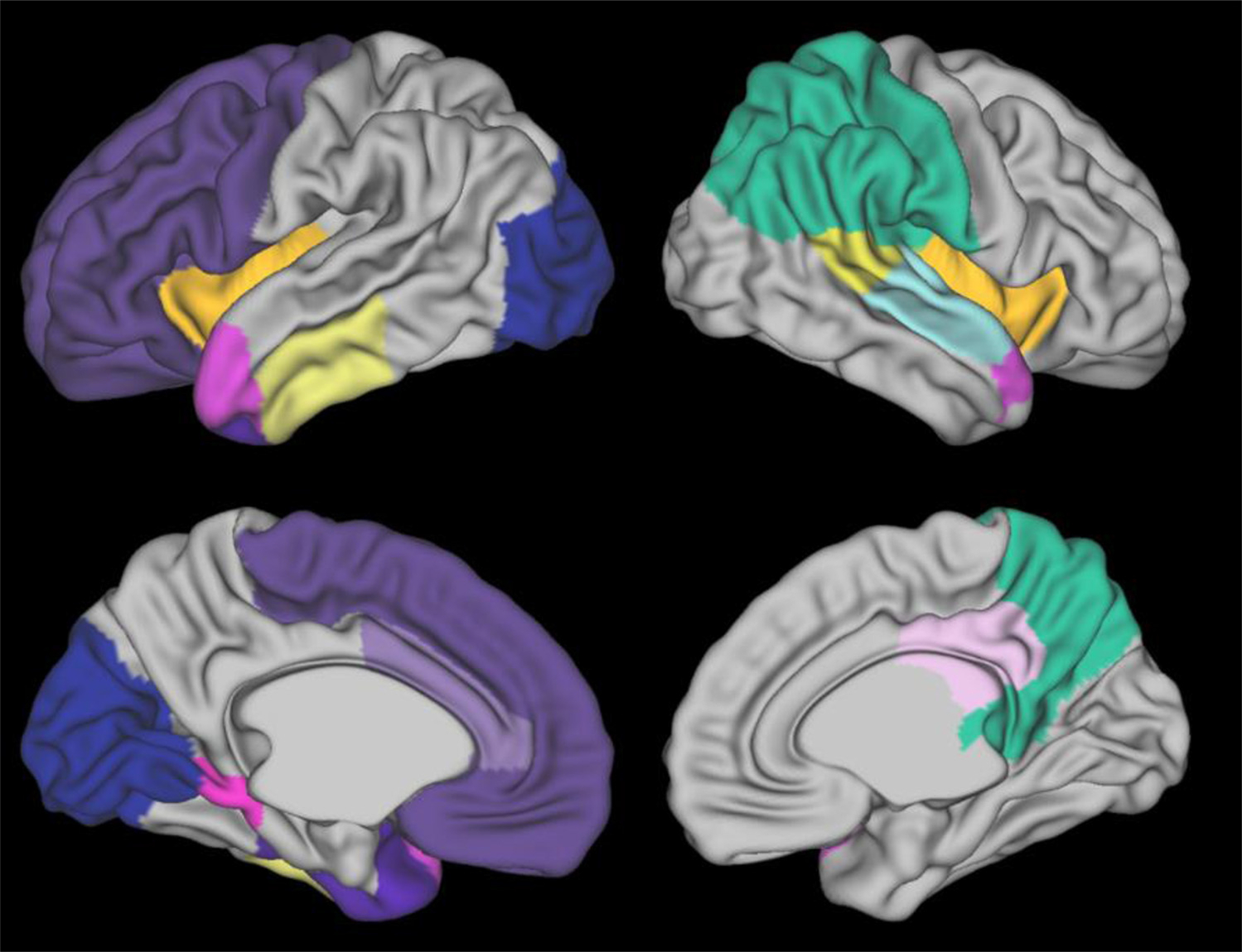
Visualization of top 15 most discriminative brain regions learned by the Ontology-guided Attribute Partitioning Ensemble Learning (OAP-EL) model.

4. Discussion

In this paper, we proposed a novel OAP approach for feature partitioning and developed an OAP-EL model for early prediction of cognitive deficits at 2 years corrected age in very preterm infants using brain maturation and geometric features of sMRI data obtained at term-equivalent age. The model was comprehensively evaluated using internal and external validations with two independent very preterm infant cohorts. Our proposed OAP-EL achieved an accuracy of 71.3%, a sensitivity of 70.6%, a specificity of 72.6%, and an AUC of 0.74 in internal validation; and an accuracy of 71.0%, a sensitivity of 70.0%, a specificity of 71.2%, and AUC of 0.71 in external validation.

4.1. Ensemble of classifiers vs. individual classifiers

Early prediction of cognitive deficits for very preterm infants continues to be a particularly challenging task in the clinical setting. Prognostic classifiers can be trained with different feature sets, and each prediction classifier has its own strengths and weaknesses. Therefore, it is natural to expect that a learning method that takes advantage of multiple classifiers would lead to superior performance. To this end, ensemble learning aims to integrate multiple classifiers to complement each other’s weaknesses, therefore rendering better performance over each individual classifier (Dong et al., 2020). The intuitive explanation of why ensemble learning works is that our human nature seeks the wisdom of crowds in making a complex decision. An example of such a decision is matching a medical treatment to a particular disease (Fitriyani et al., 2019; Raza, 2019; Mienye et al., 2020; Bhasuran and Natarajan, 2018; Yao et al., 2018). Theoretically, several reasons explain why ensemble learning works, including avoiding overfitting, greater computational efficiency, and hypothesis reinforcement (Krogh and Sollich, 1997; Yang, 2017). Our results in both internal and external validation experiments demonstrated that the ensemble of classifiers achieved significantly better prediction performance than individual classifiers.

4.2. Ensemble learning with ontology-guide feature partitioning vs. with random feature bagging

The diversity of both features and classifiers plays a key role and it is a necessary and sufficient condition in building a powerful ensemble model. A diverse set of classifiers in the base-classifier library can be trained using a diverse set of features. Most widely used feature subset partitioning schemes (e.g., attribute bagging) (Bryll et al., 2003; Ho, 1998) randomly draw feature subsets from the entire feature set, which neglects prior domain knowledge and latent relationship among features. In this study, for the first time, we proposed to integrate prior domain knowledge, expressed in ontologies, into feature a partitioning scheme. We demonstrated that the proposed ontology-guided attribute partitioning-based ensemble model produced significantly better prediction performance than the classic attribute bagging-based classifier in both internal and external validations.

4.2.1. Empirical insights of classifier ensembles via kappa-error diagram

We empirically explain the reasoning why our proposed OAP-ensemble model is better by depicting a kappa-error diagram, a visualization tool for classifier ensembles (Margineantu and Dietterich, 1997). The kappa-error diagram is a scatterplot of all pairs of classifiers in the base-classifier library of an ensemble model (i.e., each pair of base-classifiers is represented as a point on the graph). The x-coordinate of the point is a measure of diversity (denoted as K) between the outputs of the two classifiers. The pairwise K is defined as $\mathrm{K}=\frac{2(ab-bc)}{(a+b)(c+d)+(a+c)(b+d)}$, where a is the proportion of instances correctly classified by both base-classifiers, b is the proportion correctly classified by the first base-classifier but misclassified by the second one, c is the proportion misclassified by the first base-classifiers but correctly classified by the second one, and d is the proportion misclassified by both base-classifiers. The lower the K value, the more different the classifiers, and the higher chance to fill in each other’s weakness, therefore resulting in better classifier ensembles. The y-coordinate of the point is the averaged misclassification rate of the pair of classifiers. The ensemble model with k base-classifiers is represented by a “cloud” of $\frac{k(k-1)}{2}$ points, and $\frac{100k(k-1)}{2}$ points with 100 times repetition of LOOCV. Better ensembles will be the ones with a “cloud” of points near the left bottom corner of the graph (i.e., high diversity and low individual error). Fig. 14 shows that our proposed OAP-EL model produces more accurate and more diverse individual classifiers, since the “clouds” of OAP-EL are more to the left bottom corner of the graph. This indicates the key to the better overall performance we see with OAP-EL.

Fig. 14.

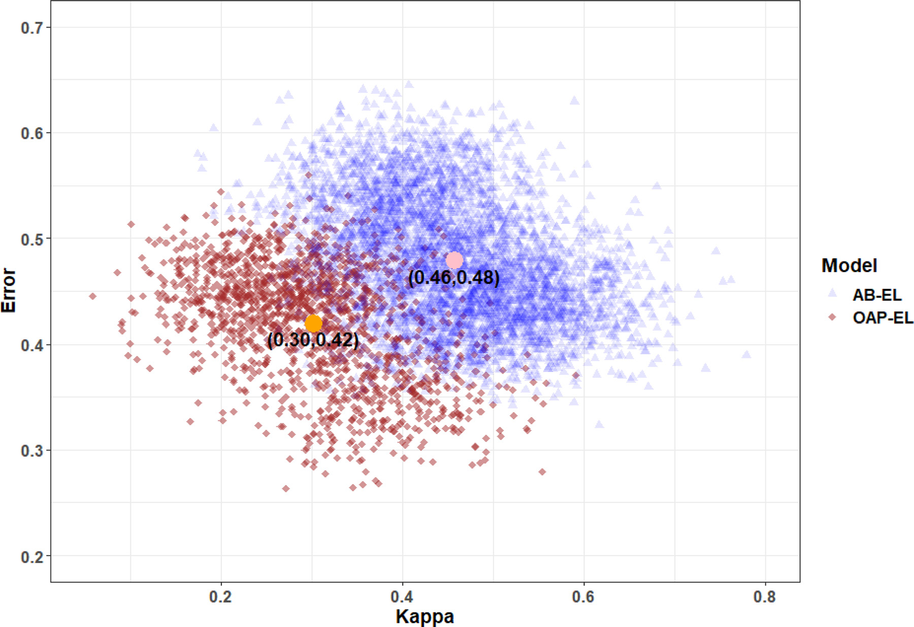
Kappa-error diagram for AB-EL and OAP-EL models. The x-coordinate of point represents the pairwise classifier diversity kappa measure, and y-coordinate is the averaged misclassification error of each pair of base-classifiers. AB-EL: Attribute Bagging Ensemble Learning; OAP-EL: Ontology-guided Attribute Partitioning Ensemble Learning. The highlight points indicate the mean of two groups.

4.3. Classifier ensemble vs. feature ensemble

The current study proposed to integrate multiple classifiers, each of which is a single-channel classifier trained using a subset of features. In contrast to this “classifier ensemble” approach, we can also train a multi-channel classifier to integrate all the feature subsets (“feature ensemble”), like what we have proposed in our prior work (Chen et al., 2019). We have demonstrated that OAP-EL model (“classifier ensemble”) performed better than OAP-mNN model (“feature ensemble”) in this particular application in both internal and external validations. Since the feature partitioning scheme was exactly the same for both models, the performance difference is likely because the multi-channel models often require a relatively large dataset to reach a converged stable training loss. The ensemble learning model has far fewer parameters, reducing the potential overfitting issue.

4.4. Impacts of imbalanced dataset

Both CINEPS and COEPS cohorts had imbalanced datasets, since very preterm infants who develop cognitive deficits were commonly fewer than the ones who develop normally. Such imbalanced datasets tend to impact two aspects of our study: model training and model evaluation. For the aspect of model training, with an imbalanced dataset, machine learning models are biased towards majority class. There are a smaller number of very preterm infants in the high-risk group compared to those in the low-risk group a the ratio of 1:2 in the CINEPS dataset. To handle this issue, we applied a data synthesis approach SMOTE-ENN that simultaneously generated new synthetic samples for minority class and randomly removed sample in the majority class that may adversely impact model learning.

For the aspect of model evaluation, we provided PR curves and calculated PRAUC for both internal and external validation. In the future clinical practice, it is better to identify correctly as many high-risk very preterm infants as possible so that early intervention can be prescribed when treatments can exert the greatest impact on prevention. PR curves would be a proper evaluation method to use when the dataset has a substantial imbalanced sample ratio. PR curves and PRAUC are able to provide a better view of model performance on positive samples in the minority class, where ROC curves and AUC might not truly reflect the model performance. In the PR curves, since the random guess baseline changes according to positive: negative sample ratios, it is critical to compare our model to the random guess baseline. In the internal validation, the positive: negative sample ratio of the CINEPS dataset is 1:2, resulting a PRAUC of 0.33 for the random guess baseline. (Figs 7, 8 and 11) Our OAP-EL model had the best PRAUC of 0.56 among all competing models. Similarly, in the external validation, the PRAUC of random guess baseline was 0.14, while the developed OAP-EL model achieved a PRAUC of 0.42, which 3 times better than the random guess baseline. (Fig. 12)

4.5. Most discriminative brain maturation and geometric features

Using the 2-level feature ranking method, we identified 15 top discriminative brain maturation and geometric features. The most predictive feature ranked by the OAP-EL model is the thickness of right insular cortex. The thickness of left insula region (ranked 13th) was also included within our feature list. Insulae are deeply buried regions that separate the frontal and parietal lobes from the temporal lobe. They are involved in a diverse array of brain functions, including perception, compassion, self-awareness, and cognitive function (Craig and Craig, 2009). Insula thickness has been positively associated with non-planning impulsivity, a widely-used measure reflecting emotional development and decision-making (Churchwell and Yurgelun-Todd, 2013). Thus, it is not surprising that our model identified insula thickness as a discriminative feature that is predictive of cognitive deficits in very preterm infants. Several other cognition-related brain regions were also identified. For example, our OAP-EL model found that the sulcal depth of the anterior part of left medial and inferior temporal gyri was significantly predictive of cognitive deficits. Previous studies have demonstrated that the middle and inferior temporal gyri are associated with language and semantic memory processing, visual perception, and multimodal sensory integration (Cabeza and Nyberg, 2000; Chao et al., 1999; Ishai et al., 1999; Tranel et al., 1997). Another highly discriminative brain region was the sulcal depth of the anterior part of left cingulate gyrus. The cingulate gyrus has been recognized to be highly involved in emotion formation and processing, learning, and memory (Tranel et al., 1997; Hadland et al., 2003; Stanislav et al., 2013). Considering the important role of the frontal lobe and occipital lobe in learning, interestingly, only one feature from each of these regions were selected by our model as top 15 discriminative features for predicting cognitive deficits. Nevertheless, because cognitive function is highly distributed across the brain, the selection of other brain regions and features that are also involved in learning and cognition suggests that our proposed OAP-EL model is able to learn meaningful brain maturation and geometric features instead of being overfitted by random noise.

4.6. Study limitations

The current study includes certain limitations. First, ontology graph construction may vary between different studies. There is no universal method regarding how to utilize domain knowledge to construct an ontology graph. In addition, we only constructed an unweighted ontology graph using prior domain knowledge. How to effectively utilize domain knowledge to construct a weighted ontology graph could be a very interesting future direction. Second, we applied a spectral graph clustering algorithm to partition features into multiple non-overlapping subsets. Partitioning features into overlapping subsets has not been considered in the current study. Third, the external validation dataset (i.e., COEPS cohort) is a small dataset, where the high-risk group only contains 10 subjects. This resulted in the fact that predictions on a few samples may cause a large variation in model performance (e.g., one correctly predicted very preterm infant may increase the sensitivity of a model from 60 to 70%). Thus, even though our model outperformed peer models in both internal and external validation in the current study, a larger external cohort is necessary to validate the generalizability of our proposed model. Finally, our OAP approach is not applicable if all features are partitioned into the same category.

5. Conclusion

We presented a novel OAP enhanced ensemble learning model integrating brain maturation and geometric features obtained at term-equivalent age for early prediction of cognitive deficits at 2 years corrected age in very preterm infants. The predictive performance of our novel ensemble model was significantly higher than models using traditional machine learning and peer ensemble learning. The proposed technique will facilitate ensemble learning in general, by helping augment the diversity among the base-classifiers. In the future, we are also interested in developing ontology aided machine learning methods to better understand and depict both brain radiomic and connectomic features.

Data and code availability

Requests to access the data sets used in this study should be directed to the corresponding author with a formal data sharing agreement and approval from the requesting researcher’s local ethics committee. The source code of the proposed model is publicly accessible on GitHub: (https://github.com/jiaolang771/aicad/tree/main/OAP_EL_Early_Prediction).

References

- Blencowe H, et al. , 2013. Born too soon: the global epidemiology of 15 million preterm births. Reprod. Health 10 (1), 1–14. [DOI] [PMC free article] [PubMed] [Google Scholar]
- Blencowe NS, et al. , 2012. Reporting of short-term clinical outcomes after esophagectomy: a systematic review. Ann. Surg. 255 (4), 658–666. [DOI] [PubMed] [Google Scholar]
- Hamilton BE, Martin JA, Osterman MJ, Curtin SC, Matthews TJ, 2015. Births: Final Data for 2014. Natl. Vital. Stat. Rep. 64 (12), 1–64. [PubMed] [Google Scholar]
- Fleiss B, Gressens P, Stolp HB, 2020. Cortical gray matter injury in encephalopathy of prematurity: link to neurodevelopmental disorders. Front. Neurol. 11, 575. [DOI] [PMC free article] [PubMed] [Google Scholar]
- Inder TE, et al. , 2005. Abnormal cerebral structure is present at term in premature infants. Pediatrics 115 (2), 286–294. [DOI] [PubMed] [Google Scholar]
- Rathbone R, et al. , 2011. Perinatal cortical growth and childhood neurocognitive abilities. Neurology 77 (16), 1510–1517. [DOI] [PMC free article] [PubMed] [Google Scholar]
- Steinman KJ, et al. , 2009. Neonatal watershed brain injury on magnetic resonance imaging correlates with verbal IQ at 4 years. Pediatrics 123 (3), 1025–1030. [DOI] [PMC free article] [PubMed] [Google Scholar]
- Bouyssi-Kobar M, et al. , 2018. Altered cerebral perfusion in infants born preterm compared with infants born full term. J. Pediatr. 193, 54–61 e2. [DOI] [PMC free article] [PubMed] [Google Scholar]
- Kline JE, et al. , 2020. Automated brain morphometric biomarkers from MRI at term predict motor development in very preterm infants. NeuroImage Clin. 28, 102475. [DOI] [PMC free article] [PubMed] [Google Scholar]
- Parikh NA, 2016. Advanced neuroimaging and its role in predicting neurodevelopmental outcomes in very preterm infants. In: Seminars in perinatology, 40 (8). WB Saunders, pp. 530–541. [DOI] [PMC free article] [PubMed] [Google Scholar]
- Kline JE, et al. , 2020. Early cortical maturation predicts neurodevelopment in very preterm infants. Arch. Dis. Child. Fetal Neonatal Ed 105 (5), 460–465. [DOI] [PMC free article] [PubMed] [Google Scholar]
- Dong X, et al. , 2020. A survey on ensemble learning. Front. Comput. Sci. 14 (2), 241–258. [Google Scholar]
- Zhang C, Ma Y, 2012. Ensemble Machine Learning: Methods and Applications. Springer. [Google Scholar]
- Bryll R, Gutierrez-Osuna R, Quek F, 2003. Attribute bagging: improving accuracy of classifier ensembles by using random feature subsets. Pattern Recognit. 36 (6), 1291–1302. [Google Scholar]
- Ho TK, 1998. The random subspace method for constructing decision forests. IEEE Trans. Pattern Anal. Mach. Intell. 20 (8), 832–844. [Google Scholar]
- Kuncheva LI, et al. , 2010. Random subspace ensembles for FMRI classification. IEEE Trans. Med. Imaging 29 (2), 531–542. [DOI] [PubMed] [Google Scholar]
- Grüninger M and Fox MS, Methodology for the design and evaluation of ontologies. 1995.
- Staab S, et al. , 2001. Knowledge processes and ontologies. IEEE Intell. Syst. 16 (1), 26–34. [Google Scholar]
- Uschold M, Gruninger M, 1996. Ontologies: Principles, methods and applications. Knowl. Eng. Rev. 11 (2), 93–136. [Google Scholar]
- Consortium GO, 2004. The gene ontology (GO) database and informatics resource. Nucleic Acids Res. 32 (suppl_1), D258–D261. [DOI] [PMC free article] [PubMed] [Google Scholar]
- Kulmanov M, Smaili FZ, Gao X, Hoehndorf R (2020). Machine learning with biomedical ontologies. biorxiv. [Google Scholar]
- Smith B, et al. , 2005. Relations in biomedical ontologies. Genome Biol. 6 (5), 1–15. [DOI] [PMC free article] [PubMed] [Google Scholar]
- Zhang SB, Tang QR, 2016. Protein–protein interaction inference based on semantic similarity of gene ontology terms. J. Theor. Biol. 401, 30–37. [DOI] [PubMed] [Google Scholar]
- Shen Y, et al. , 2018. An ontology-driven clinical decision support system (IDDAP) for infectious disease diagnosis and antibiotic prescription. Artif. Intell. Med. 86, 20–32. [DOI] [PubMed] [Google Scholar]
- Köhler S, et al. , 2009. Clinical diagnostics in human genetics with semantic similarity searches in ontologies. Am. J. Hum. Genet. 85 (4), 457–464. [DOI] [PMC free article] [PubMed] [Google Scholar]
- Makropoulos A, et al. , 2018. The developing human connectome project: a minimal processing pipeline for neonatal cortical surface reconstruction. NeuroImage 173, 88–112. [DOI] [PMC free article] [PubMed] [Google Scholar]
- Gousias IS, et al. , 2012. Magnetic resonance imaging of the newborn brain: manual segmentation of labelled atlases in term-born and preterm infants. NeuroImage 62 (3), 1499–1509. [DOI] [PubMed] [Google Scholar]
- Chen T, Guestrin C, 2016. XGBoost: a scalable tree boosting system. In: Proceedings of the 22nd ACM SIGKDD International Conference on Knowledge Discovery and Data Mining. [Google Scholar]
- Parikh NA, et al. , 2021. Perinatal risk and protective factors in the development of diffuse white matter abnormality on term-equivalent age magnetic resonance imaging in infants born very preterm. J. Pediatr. 233, 58–65 e3. [DOI] [PMC free article] [PubMed] [Google Scholar]
- Logan J, et al. , 2021. Adverse effects of perinatal illness severity on neurodevelopment are partially mediated by early brain abnormalities in infants born very preterm. J. Perinatol. 41 (3), 519–527. [DOI] [PMC free article] [PubMed] [Google Scholar]
- Bayley N, 2006. Bayley Scales of Infant and Toddler Development: Bayley-III. Harcourt Assessment Psych. Corporation. [Google Scholar]
- Tustison NJ, et al. , 2010. N4ITK: improved N3 bias correction. IEEE Trans. on Med. Imaging 29 (6), 1310–1320. [DOI] [PMC free article] [PubMed] [Google Scholar]
- Smith SM, 2002. Fast robust automated brain extraction. Hum. Brain Mapp. 17 (3), 143–155. [DOI] [PMC free article] [PubMed] [Google Scholar]
- Makropoulos A, et al. , 2014. Automatic whole brain MRI segmentation of the developing neonatal brain. IEEE Trans. Med. Imaging 33 (9), 1818–1831. [DOI] [PubMed] [Google Scholar]
- Schuh A, et al. , 2017. A deformable model for the reconstruction of the neonatal cortex. In: Proceedings of the 2017 IEEE 14th International Symposium on Biomedical Imaging (ISBI 2017). IEEE. [Google Scholar]
- Shi J, Malik J, 2000. Normalized cuts and image segmentation. IEEE Trans. Pattern Anal. Mach. Intell. 22 (8), 888–905. [Google Scholar]
- Chawla NV, et al. , 2002. SMOTE: synthetic minority over-sampling technique. J. Artif. Intell. Res. 16, 321–357. [Google Scholar]
- Batista GE, Prati RC, Monard MC, 2004. A study of the behavior of several methods for balancing machine learning training data. ACM SIGKDD Explor. Newsl. 6 (1), 20–29. [Google Scholar]
- Fix E, Hodges JL, 1989. Discriminatory analysis. Nonparametric discrimination: consistency properties. Int. Stat. Rev 57 (3), 238–247 /Revue Internationale de Statistique. [Google Scholar]
- Cox DR, 1958. The regression analysis of binary sequences. J. R. Stat. Soc. Ser. B 20 (2), 215–232 (Methodological). [Google Scholar]
- Cortes C, Vapnik V, 1995. Support-vector networks. Mach. Learn. 20 (3), 273–297. [Google Scholar]
- Wu X, et al. , 2008. Top 10 algorithms in data mining. Knowl. Inf. Syst. 14 (1), 1–37. [Google Scholar]
- Ho TK, 1995. Random decision forests. In: Proceedings of the 3rd International Conference on Document Analysis and Recognition. IEEE. [Google Scholar]
- McCulloch WS, Pitts W, 1943. A logical calculus of the ideas immanent in nervous activity. Bull. Math. Biophys. 5 (4), 115–133. [PubMed] [Google Scholar]
- Dietterich TG, 2002. Ensemble learning. In: The Handbook of Brain Theory and Neural Networks, 2. The MIT Press, pp. 110–125. [Google Scholar]
- Breiman L, 1996. Bagging predictors. Mach. Learn. 24 (2), 123–140. [Google Scholar]
- Wolpert DH, 1992. Stacked generalization. Neural Netw. 5 (2), 241–259. [Google Scholar]
- Chen M, et al. , 2019. A multichannel deep neural network model analyzing multiscale functional brain connectome data for attention deficit hyperactivity disorder detection. Radiol. Artif. Intell. 2 (1), e190012. [DOI] [PMC free article] [PubMed] [Google Scholar]
- Azhagusundari B, Thanamani AS, 2013. Feature selection based on information gain. Int. J. Innov. Technol. Explor. Eng. 2 (2), 18–21 (IJITEE). [Google Scholar]
- Fitriyani NL, et al. , 2019. Development of disease prediction model based on ensemble learning approach for diabetes and hypertension. IEEE Access 7, 144777–144789. [Google Scholar]
- Raza K, 2019. Improving the prediction accuracy of heart disease with ensemble learning and majority voting rule. In: U-Healthcare Monitoring Systems. Elsevier, pp. 179–196. [Google Scholar]
- Mienye ID, Sun Y, Wang Z, 2020. An improved ensemble learning approach for the prediction of heart disease risk. Inf. Med. Unlocked 20, 100402. [Google Scholar]
- Bhasuran B, Natarajan J, 2018. Automatic extraction of gene-disease associations from literature using joint ensemble learning. PloS One 13 (7), e0200699. [DOI] [PMC free article] [PubMed] [Google Scholar]
- Yao D, et al. , 2018. An ensemble learning system for a 4-way classification of Alzheimer’s disease and mild cognitive impairment. J. Neurosci. Methods 302, 75–81. [DOI] [PMC free article] [PubMed] [Google Scholar]
- Krogh A, Sollich P, 1997. Statistical mechanics of ensemble learning. Phys. Rev. E 55 (1), 811. [Google Scholar]
- Yang Y, 2017. Ensemble learning. In: Temporal Data Mining Via Unsupervised Ensemble Learning. Elsevier, pp. 35–56. [Google Scholar]
- Margineantu DD, Dietterich TG, 1997. Pruning adaptive boosting. ICML. Citeseer. [Google Scholar]
- Craig AD, Craig A, 2009. How do you feel–now? The anterior insula and human awareness. Nat. Rev. Neurosci. 10 (1). [DOI] [PubMed] [Google Scholar]
- Churchwell JC, Yurgelun-Todd DA, 2013. Age-related changes in insula cortical thickness and impulsivity: significance for emotional development and decision-making. Dev. Cogn. Neurosci. 6, 80–86. [DOI] [PMC free article] [PubMed] [Google Scholar]
- Cabeza R, Nyberg L, 2000. Imaging cognition II: An empirical review of 275 PET and fMRI studies. J. Cogn. Neurosci. 12 (1), 1–47. [DOI] [PubMed] [Google Scholar]
- Chao LL, Haxby JV, Martin A, 1999. Attribute-based neural substrates in temporal cortex for perceiving and knowing about objects. Nat. Neurosci. 2 (10), 913–919. [DOI] [PubMed] [Google Scholar]
- Ishai A, et al. , 1999. Distributed representation of objects in the human ventral visual pathway. Proc. Natl. Acad. Sci. 96 (16), 9379–9384. [DOI] [PMC free article] [PubMed] [Google Scholar]
- Tranel D, Damasio H, Damasio AR, 1997. A neural basis for the retrieval of conceptual knowledge. Neuropsychologia 35 (10), 1319–1327. [DOI] [PubMed] [Google Scholar]
- Tranel D, Damasio H, Damasio AR, 1997. Cingulate binds learning. Trends Cogn. Sci. 1 (1), 2. [DOI] [PubMed] [Google Scholar]
- Hadland K, et al. , 2003. The effect of cingulate lesions on social behaviour and emotion. Neuropsychologia 41 (8), 919–931. [DOI] [PubMed] [Google Scholar]
- Stanislav K, et al. , 2013. Anatomical characteristics of cingulate cortex and neuropsychological memory tests performance. Procedia Soc. Behav. Sci. 86, 128–133. [Google Scholar]
Associated Data
This section collects any data citations, data availability statements, or supplementary materials included in this article.
Supplementary Materials
Data Availability Statement