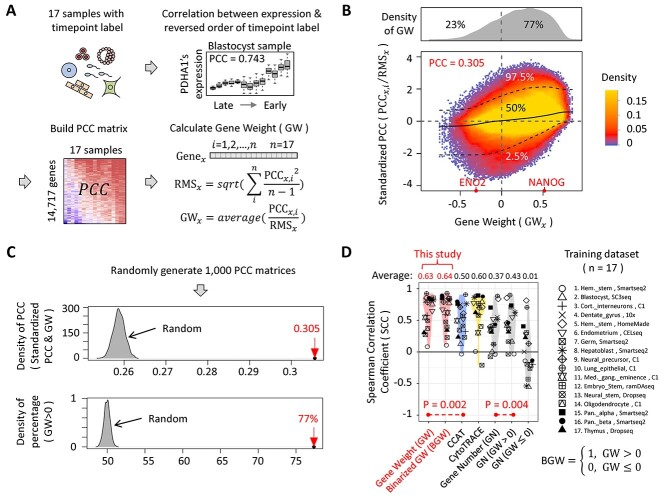
Figure 2.

The generation of GW and the discovery of BGW. (A) The workflow of generating GW. ‘PCC’ stands for Pearson Correlation Coefficient. ‘RMS’ stands for Root-Mean-Square that is calculated by using the ‘scale’ function in R. In this study, the term ‘sample’ indicates the constructed sample that contains all scRNA-seq data of a previously published dataset. (B) The scatter plot describing the relationship between GW values and standardized PCCs. For each gene, we build two vectors. The first vector (y axis) has 17 elements that are the standardized PCCs of 17 training samples, whereas the second vector (x axis) has 17 elements sharing the same value (the GW value of the given gene). The upper dot-line, middle line and lower dot-line are the 97.5%, 50% and 2.5% quintiles of standardized PCCs, respectively. The color on the scatter plot indicates the density of points, whereas the upper gray panel shows the density plot of GW values. (C) Two characteristics of GW. We calculate 1000 random GW sets by randomly generating 1000 PCC matrices. The gray areas represent the distribution of statistics of the random GW sets, whereas the red arrows highlight the statistics of the real GW set. (D) The comparison results using training dataset. ‘GN’ means that we define DP as the number of detected genes. ‘GN (GW > 0)’ and ‘GN (GW ≤ 0)’ mean that we define DP as the number of detected genes with positive GW and negative GW (there is no GW that is equal to 0), respectively.