

Abstract
The existing slime mould algorithm clones the uniqueness of the phase of oscillation of slime mould conduct and exhibits slow convergence in local search space due to poor exploitation phase. This research work exhibits to discover the best solution for objective function by commingling slime mould algorithm and simulated annealing algorithm for better variation of parameters and named as hybridized slime mould algorithm–simulated annealing algorithm. The simulated annealing algorithm improves and accelerates the effectiveness of slime mould technique as well as assists to take off from the local optimum. To corroborate the worth and usefulness of the introduced strategy, nonconvex, nonlinear, and typical engineering design difficulties were analyzed for standard benchmarks and interdisciplinary engineering design concerns. The proposed technique version is used to evaluate six, five, five unimodal, multimodal and fixed-dimension benchmark functions, respectively, also including 11 kinds of interdisciplinary engineering design difficulties. The technique’s outcomes were compared to the results of other on-hand optimization methods, and the experimental results show that the suggested approach outperforms the other optimization techniques.
Keywords: CEC-2005, Hybrid search algorithms, Metaheuristics search, Engineering optimization
Introduction
Nowadays, the usage of metaheuristic algorithms has become widespread in numerous applied fields because of their advanced presentation with less computing duration than other determinant algorithms in dissimilar optimization issues [1]. Uncomplicated conceptions are necessary to attain good outcomes, as well it is effortless to immigrate to dissimilar disciplines. In addition, the need for randomness in a while period of a few determinant algorithms prepares it leaning to go under local optima, and random parameters in metaheuristics make the algorithms explore for every optimum finding in search space, therefore, efficiently escaping local optimum. According to [2], the stochastic algorithms are less efficient than gradient descent algorithms for using gradient information. It is noticed that gradient descent algorithms have the convergence speed quicker than metaheuristic methods. On the other hand, a metaheuristics algorithm classically begins the optimization procedure at randomly produced outcomes and does not require gradient information, thus composing the algorithm extremely appropriate for realistic complications when the derivative data are not known. In reality, the solution location of several issues is repeatedly undetermined or endless. This might be impossible to bring out optimum solutions by bisecting the solution location over existing situations. Metaheuristics algorithms notice the immediate optimum solution of the issue by examining a huge solution space in random by sure means, to discover or produce enhanced solutions for the optimization issue over inadequate conditions or computational ability [3].
In context to the above discussions, an intermingle variant slime mould optimization algorithm was introduced using a simulated annealing technique into the planned research work, and the suggested hybrid translation of population-based metaheuristics search technique was examined to unravel the unique standard customary benchmark issues: unimodal, multimodal, fixed dimensions. Apart from this, the suggested optimizer’s performance was evaluated for engineering design and optimization problems for a more thorough investigation.
Earlier to this article, a few researchers introduced the same algorithm; however, the mode of idea of the algorithm and handling outline is quite diverse from the algorithms suggested in this article. A hybrid optimizer adaptive β hill climbing was combined with slime mould algorithm, here slime mould algorithm is in addition strengthened with Brownian motion and tournament selection to improve exploration capabilities thus producing better quality outcomes in the exploitation phase [4]. Zheng-Ming Gao et al. [5] introduced a technique named grey wolf optimizer–slime mould algorithm (GWO-SMA) to minimize the influence of uncertainty as low as probable which is best suited for a few benchmark functions and not suggested for engineering design issues. Juan Zhao et al. [6] proposed an improved slime mould algorithm with Levy flights and observed that when improved SMA is replaced with uniformly distributed factor, it performed well and when improved SMA is replaced with Gauss Distributed factor, it stuck in local minima. Juan et al. [7] promoted the Chaotic SMA–Chebyshev map and observed its performance to be a better, stable, more rapid, and better choice to apply in real engineering issues. Levy flight–slime mould (LF-SMA) algorithm [8] is clout by the actions of slime mould which is further mixed up with Levy distribution and excelled in obtaining better results in the exploration phase. Improved slime mould algorithm (ISMA) is developed from traditional SMA in two aspects: the exploration phase is aided with a modified opposition-based learning technique as well the phase of exploitative is aided with Nelder–Mead simplex search method to adjust the parameters of the controllers to control the velocity of a DC motor by a fractional-order PID (FOPID) controller as well as requires to maintain the automatic voltage regulator (AVR) at its level of terminal voltage through a PID in addition with second-order derivative (PIDD2) controller [9]. The combination of slime mould and Harris hawks optimization (HHO-SMA) implemented in [10] stood better technique to improve slow convergence speed. The improved version of slime mould with cosine controlling parameters in [11] could abolish errors as well as give better outcomes in engineering design issues. Accordingly, [12] finds the solution to a single solution optimization issue by replicating the 5 existence series of amoeba Dictyostelium discoideum: a phase of vegetative, aggregative, mound, slug, and dispersal using ε-ANN to build an initiative stage. To assess the Pareto optima solutions, the authors in [13] suggested multi-objective slime mould algorithm (MOSMA) for better convergence in association with elitist non-dominated sorting method. Considering two forms of slime mould arrangement [14] introduced a technique to build a wireless sensor setup to correlate two distinct local routing protocols. The network named Physarum is united with the ant colony model to enhance the technique’s proficiency to escape confined optimum values to treat the migrating agent issue efficiently [15]. Motivated by the dissemination of slime mould, Schmickland [16] suggested a bio-motivated navigation method framed for swarm robotics. Promotion of inexpensive and fault-tolerant charts based on foraging procedure of slime mould is done in [17]. According to above conversation, the majority of the pattern slime mould methods have been worn graph theory as well as in generation networks. Thus, the nature of this creature influenced scholars in the field of graph optimization [18]. Monismith et al. [12] simulated the life cycle of amoeba Dictyostelium discoideum to utilize the developed algorithm to optimize the issue with less experimental proofs.
With a unique pattern, a hybrid combination hSMA-SA introduced in this work primarily mimics the nature of slime mould’s foraging as well as morphological transforms. Meanwhile, the usage of adaptive weights in SMA simulates in producing positive and negative feedback throughout foraging, hence creating three diverse morphotypes. The simulated annealing algorithm is intermixed to boost the phase of exploitation of classical SMA resulting in improved results of the suggested hSMA-SA technique and proved better than already existing techniques. Overall, this approach is easier to use than prior population-based algorithms and requires fewer operators by least amount of computational struggles. The left behind parts of the current article enclose a literature review; background of suggested work in the next section; concepts of conventional slime mould algorithm (SMA), simulated annealing algorithm (SA), and the suggested hybrid hSMA-SA technique are discussed in the third section. The fourth section describes the standard benchmark functions. The fifth section displays the findings and compares them to those of other methods. In part 6, test on 11 engineering-based optimization design challenges has been carried, and the last section stands for the paper’s conclusion, limits, and future scope.
Literature review
Single-based and population-based metaheuristics are two types of metaheuristic algorithms. According to the names addressed, the former case has only one solution in the whole optimization process, whereas in the latter case, a bunch of solutions is developed in every iteration of optimization. In population-based techniques, an optimal or suboptimal solution may be taken into consideration, which may be as similar as the optimal or precinct location. These population metaheuristics techniques frequently emulate nominal phenomena. These types of techniques usually start the procedure of optimization by developing a bunch of individuals (population), in which every individual of the population reflects an aspirant optimum solution. Accordingly, the population progress iteratively by making use of stochastic functions at times to reinstate the present population with a newly developed population. This procedure comes to an end unless and until the simulation process gets satisfied with end command.
Metaheuristics algorithms are naturally motivated by actual-world phenomenality to bring out improved solutions for optimization issues by resembling physical laws or biological experience. The physics-based techniques are those which applies mathematical conventions or techniques which includes sine cosine algorithm (SCA) [19], gravitational search algorithm (GSA) [20], central force optimization (CFO) [21, 22], charged system search (CSS) [23], and multi-verse optimizer (MVO) [24]. The two major classes of metaheuristic algorithms are evolutionary techniques and swarm intelligent methods which are nature-influenced strategies. The insight of the evolutionary algorithm emanates from the progression of biological fruition in environment, which when analyzed with conventional optimization algorithms; this is a global optimization technique having well robustness and appropriateness. The prevalent algorithms in the group of evolutionary algorithms are: genetic programming (GP) [25], evolutionary programming (EP) [26], biogeography-based optimization (BBO) [27] which helped in analyzing biological species geographical distribution, and explained how these can be utilized to infer techniques appropriate for optimization. Differential evolution (DE) [28] is an evolutionary algorithm which includes genetic algorithms, evolutionary strategies and evolution programming. Evolutionary programming (EP) and genetic algorithm (GA) [29] are haggard from Darwinian Theory and Evolution Strategy (ES) [30]. The purpose of EP, ES, and swarm-intelligence techniques in logical research, and real-time issues are wide-ranging rapidly [31].
Swarm intelligence (SI) [32] encompasses a joint or communal intellect that unnaturally replicates the devolution of a biological bundle in the environment or the combined mannerisms of self-arranging structures. In this group of algorithms, the idea originates from biological communities present in the environment that have cooperative deeds and cleverness to accomplish an assured function. Reputable and current techniques in this set are particle swarm optimization (PSO) [33], moth flame optimization (MFO) [34], artificial bee colony (ABC) [35], Harris hawks optimizer (HHO) [36], fruit fly optimization algorithm (FFOA) [37], ant colony optimization (ACO) [38], and grey wolf optimization (GWO) [39]. Human-based techniques are those which resemble the activities of human works. In this group of algorithms, the inspiration starts from human activity in an assigned work that supports to finish the function assured. Teaching–learning-based optimization (TLBO) [40] imitates the teaching–learning procedure in a classroom, and tabu search (TS) [41]. A graphical diagram for the categorization of evolutionary and SI techniques is depicted in Fig. 1a and b displaying the history timeline of the other metaheuristic algorithms enclosed in this review. Table 1 showcases the last decade from the year (2012–2022) which exhibits the investigative works on finding solutions for numerical and engineering design problems.
Fig. 1.

a Categories of SI and evolutionary methods. b Timeline of metaheuristics. TLBO teaching–learning-based optimization, KH krill herd, FP flower pollination, CSO cuckoo search algorithm, CSPSO cuckoo search particle swarm optimization, CSLF cuckoo search–Levy flight, PeSO penguins search optimization, FA firefly algorithm, BA bat algorithm, GWO grey wolf optimizer, FOA forest optimization algorithm, BHA black hole algorithm, MFO moth flame optimizer, SFSA stochastic fractal search algorithm, CSA crow search algorithm, LOA lion optimization algorithm, SCA sine cosine algorithm, GWO-SCA hybrid grey wolf optimizer and sine cosine algorithm, CSAHC cuckoo search algorithm with hill climbing, IBO Chaos improved butterfly algorithm with chaos, Hybrid ABC/MBO artificial bee colony with monarch butterfly optimization, TGA tree growth algorithm, IHFA improved hybrid firefly algorithm, HHO Harris hawks optimizer, EPC emperor penguins colony, HGSO Henry gas solubility optimization, PSA particle swarm optimization, MOSMA multi-objective slime mould algorithm, GWO-SMA hybrid grey wolf optimization–slime mould algorithm, AHO archerfish hunting optimizer, AQ Aquila optimizer, AOA arithmetic optimization algorithm, AVOA African vultures optimization algorithm, CHHO chaotic Harris hawks optimizer, MOHHOFOA multi-objective Harris hawks optimization fruit fly optimization algorithm, GTO gorilla troops optimization, GTOA modified group theory-based optimization algorithm, CryStAl crystal structure optimization, SOA seagull optimization algorithm, CSOA criminal search optimization algorithm
Table 1.
A look into population metaheuristics in a nutshell
| Technique and its reference number | Name of the author and year | A quick summary |
|---|---|---|
| Seagull optimization algorithm (SOA) [55] | Yanhui Che and Dengxu He 2022 | This paper proposed an enhanced seagull optimization algorithm to eliminate the defects of traditional seagull optimizer. The technique is tested on 12 various engineering optimization problems |
| Modified group theory-based optimization algorithms for numerical optimization (GTOA) [56] | Li et al. 2022 | This paper concentrated on studying the applicability of the proposed GTOA to solve optimization problems by introducing two versions of GTOA which uses binary coding and integer coding. The performance proved to obtain better convergence rate and average accuracy |
| Criminal search optimization algorithm (CSOA) [57] | Srivastava et al. 2022 | This paper introduced criminal search optimization algorithm which has been developed based on intelligence of policemen in catching a criminal. The presentation of the technique has been evaluated on standard benchmark functions—CEC-2005 and CEC-2020. Five test cases have been operated to measure the results of the suggested algorithm with other techniques and proved the good |
| Crystal structure optimization approach to problem-solving in mechanical engineering design (CryStAl) [58] | Babak Talatahari et al. 2022 | The authors of this paper introduced a metaheuristic named crystal structure algorithm to discover solutions for engineering mechanics and design problems. Further, the technique has been examined on 20 benchmark mathematical functions and obtained satisfying outputs when measured with other existing methods |
| African vultures optimization algorithm (AVOA) [59] | Abdollahzadeh et al. 2021 | The authors of this paper proposed African vultures optimization algorithm imitating the living style of African vultures foraging and navigation attitude. First, the method’s feat is tested on 36 benchmark functions and its applicability is announced on finding optimum solutions for 11 engineering design problems |
| Flow direction algorithm (FDA) [60] | Hojat Karami et al. 2021 | This paper focused in proposing a physics-based algorithm named Flow direction algorithm imitating flow direction in a drainage basin. The method has been tested on 13, 10 and 5 classical mathematical, new mathematical benchmark functions and engineering design problems, respectively. These results proved better than other techniques results |
| A new hybrid chaotic atom search optimization based on tree-seed algorithm and Levy flight for solving optimization problems [61] | Saeid et al. 2021 | The authors in this papers used combination of metaheuristic algorithms to crack 7 special engineering issues. This atom search algorithm convergence speed is enhanced by chaotic maps as well as Levy flight random walk. Furthermore, tree-seed method ties with ASO. These combinations of algorithms yield good results |
| A multi-objective optimization algorithm for feature selection problems (MOHHOFOA) [62] | Abdollahzadeh et al. 2021 | The authors in this paper used three different solutions for feature selection. First, Harris hawks optimization algorithm is multiplied; second, fruit fly optimization algorithm is multiplied, and in third stage, these two algorithms have been hybridized to locate solutions for feature selection issues |
| Arithmetic optimization algorithm (AOA) [63] | Laith et al. 2021 | This paper proposed arithmetic optimization algorithm and tested its performance on 29 benchmark functions 7 real-world engineering design problems. The outcomes obtained by this technique proved better among other existing methods |
| Aquila optimizer (AO) [64] | Laith Abualigah et al. 2021 | The authors suggested population-based optimization method named Aquila optimizer to solve optimization problems. The technique has been evaluated on 23 benchmark functions and 7 real-life engineering design issues. The outcomes are good than other methods |
| Artificial gorilla troops optimizer (GTO) [65] | Abdollahzadeh et al. 2021 | The authors in this paper proposed Artificial gorilla troops optimizer which is designed to improve the phases of exploration and exploitation. The algorithm is examined on 52 functions and 7 engineering design problems |
| Binary slime mould algorithm (BSMA) [66] | Abdel et al. 2021 | This paper proposed slime mould algorithm with 4 binary versions for feature selection. All these versions were tested on 28 datasets of UCI repository |
| 1D SMA models (SMAs) [67] | Sonia Marfia et al. 2021 | This paper elevates the SMA 1D models to elucidate response of SMAs in thermo mechanical models |
| Slime mould algorithm (SMA) [68] | Davut Izci et al. 2021 | Tested on several benchmark functions. Using PID controllers, the capability of SMA optimization is enhanced |
| Hybrid improved slime mould algorithm with adaptive β hill climbing (BTβSMA) [4] | Kangjian Sun et al. 2021 | Tested on 16 benchmark functions and is suggested to lighten the unfledged global and local hunt in standard SMA |
| Archerfish hunting optimizer (AHO) [69] | Farouq Zitouni et al. 2021 | Tested on 10 benchmark functions, 5 engineering problems. AHO replicates the behavior of Archerfish like jumping and shooting to find closer optimum values |
| WLSSA [70] | Hao Ren et al. 2021 | Tested on 23 benchmark functions. With the combination of slap swarm and weight adaptive Levy flight have noticed finer optimum values |
| Multi-temperature simulated annealing algorithm (MTSA) [71] | Shih-Wei-Lin et al. 2021 | This algorithm is developed to reduce the scheduling issues which influence the design and optimization of automated systems |
| Self-adaptive salp swarm algorithm (SASSA) [72] | Rohith Salgotra et al. 2021 | Salp swarm algorithm is improved to mould it into self-adaptive by supplementing it by four modifications which possess in improving local search |
| Simulated annealing with Gaussian mutation and distortion equalization algorithm (SAGMDE) [73] | Julian Lee et al. 2020 | This combined algorithm applied on different data sets yields better results in exploratory phase when only simulated annealing algorithm was applied |
| Slime mould algorithm (SMA) [3] | Shimin Li et al. 2020 |
Tested on 33 benchmark functions It replicated the characteristics of slime mould. SMA, intended to give better exploration capability and extending its application in kernel extreme learning machine |
| Hybrid grey wolf optimization–slime mould algorithm (GWO-SMA) [5] | Zheng-Ming Gao et al. 2020 | Made 3 types of experiments resulting it did not give better results in combining GWO and SMA. SMA equations were unique and excellent and firm to progress |
| Chaotic SMA–Chebyshev map [7] | Juan Zhao et al. 2020 | Tested on standard benchmark functions and noticed the results to be better and the technique performed faster with stability |
| Improved slime mould algorithm with Levy flight [6] | Juan Zhao et al. 2020 | Worked to reduce the pressure of randomness and noticed SMA–Levy flight with uniform distributed parameters would give better results |
| Modified slime mould algorithm via Levy flight [8] | Zhesen Cui et al. 2020 | Tested on 13 benchmark functions and 1 engineering design issue and notice the results obtained were better and steady |
| Hybridized Harris hawks optimization and slime mould algorithm (HHO-SMA) [10] | Juan Zhao et al. 2020 | The research attentively made efforts on many updating discipline mostly individuals on swarms |
| Improved slime mould algorithm with cosine controlling parameter [11] | Zheng-Ming Gao et al. 2020 | The research helped in finding that the controlling parameters are very essential for the technique to perform better, at the same time noticed that all parameters were not acceptably helpful. Hence, should find more apt method |
| Multi-objective slime mould algorithm based on elitist non-dominated sorting (MOSMA) [13] | Manoharan Premkumar et al. 2020 | Tested on 41 various cases, constrained, unconstrained as well as on real-life engineering issues. On applying this algorithm resulted in high-quality and effectiveness solutions for tough multi-objective issues |
| PSA: a photon search algorithm [74] | Y. Liu and Li 2020 | 23 functions were put to the test. The characteristics of photons in physics were the inspiration for this piece. The algorithm has strong global search and convergence capabilities |
| Movable damped wave algorithm [75] | Rizk et al. 2019 | This paper proposed movable damped wave algorithm and the algorithm has been examined on 23 benchmark functions and 3 engineering design problems |
| Henry gas solubility optimization: a novel physics-based algorithm (HGSO) [76] | Hashim et al. 2019 | 47 benchmark functions were used in the testing. It is modeled after Henry’s reign. HGSO, which aims to meet the check room and halt optima locale’s production and conservation capacities |
| Emperor penguins colony (EPC) [77] | Sasan et al. 2019 | A new metaheuristic algorithm named emperor penguins colony is proposed in this paper and has been tested on 10 benchmark functions |
| Harris hawks optimization (HHO) [78] | Heidari et al. 2019 | There were 29 benchmarks and 6 technical issues which were tested on. It is being introduced to help with various optimization chores. Nature’s cooperative behaviors, as well as the patterns of predatory birds hunting Harris’ hawks, impact the strategy |
| Tree growth algorithm (TGA) [79] | Armin et al. 2018 | The authors introduced Tree growth algorithm which is inspired by trees competition for acquiring light and food. It has been examined on 30 benchmark functions and 5 engineering design problems |
| Hybrid artificial bee colony with monarch butterfly optimization [80] | Waheed et al. 2018 | This paper introduced a new algorithm named hybrid ABC/MBO (HAM) and evaluated on 13 benchmark functions and proved better in outcomes |
| An improved hybrid firefly algorithm for solving optimization problems (IHFA) [81] | Fazli Wahid et al. 2018 | This paper introduced a novel method called GA-FA-PS algorithm and tested on 3 benchmark functions and proved that the obtained results are better than firefly algorithm and genetic algorithm |
| An improved butterfly optimization algorithm with chaos [82] | Sankalap Arora et al. 2017 | The authors in this paper improved butterfly optimization with chaos to increase its performance to avoid local optimum and convergence speed. The suggested chaotic BOAs are validated 3 benchmark functions and 3 engineering design problems |
| Cuckoo search algorithm–hill climbing technique (CSAHC) [83] | Shehab et al. 2017 | The authors proposed new cuckoo search algorithm by hybridizing with hill climbing technique to solve optimization issues. It has been examined on 13 benchmark functions and proved successful |
| Hybrid GWO-SCA [84] | Singh et al. 2017 | This paper proposed hybrid grey wolf optimizer and sine cosine technique and tested on 22 functions, 5 bio-medical dataset and 1 sine dataset problems |
| SCA: a sine cosine algorithm for solving optimization problems [85] | Seyedali Mirjalili 2016 | The author proposed SCA for the solutions of optimization problems and its efficiency is validated on testing 19 benchmark functions |
| Lion optimization algorithm (LOA): a nature-inspired metaheuristic algorithm [86] | Maziar Yazdani et al. 2016 | This paper introduced Lion optimization algorithm and has been examined on 30 benchmark functions |
| Crow search algorithm (CSA) [87] | Alireza Askarzadeh 2016 | The author proposed crow search algorithm and applied to unravel 6 engineering design issues. The outputs were promising than existing methods |
| Stochastic fractal search: a powerful metaheuristic algorithm (SFS) [88] | Salimi 2015 | Uni, multi, fixed functions, and engineering functions were all tested |
| Moth flame optimization algorithm: a novel nature-inspired heuristic paradigm (MFO) [34] | Mirjalili 2015 | 7 engineering designs were tested, as well as 29 benchmarks. This optimizer followed navigation tactic of moth flame. The outcomes of this method stood better than existing techniques |
| Solving optimization problems using black hole algorithm (BHA) [89] | Masoum Farahmandian et al. 2015 | This paper suggested black hole algorithm and has been checked on 19 benchmark functions. These results were better than PSO and GA |
| Forest optimization algorithm FOA [90] | Ghaemi et al. 2014 | This technique is for determining the utmost as well as minimum value using a practical appliance, as well as demonstrating that the FOA can generally solve that are acceptable |
| Grey wolf optimizer (GWO) [39] | Mirjalili, Mirjalili, and Lewis 2014 | The researchers looked at 29 BFs and 3 optimization engineering-based approaches. The image was enthused by a swarm-intelligence optimization and was inspired by grey wolves. Grey wolves’ communal structure and hunting conduct were used to develop the suggested model |
| Cuckoo search algorithm using Lèvy flight: a review [91] | Sangita Roy et al. 2013 | The authors in this paper discussed about cuckoo search algorithm using Levy flight algorithm and noticed that the presentation of this method is superior to particle swarm optimizer and genetic algorithm when examined on 10 benchmark functions |
| Firefly algorithm: recent advances and applications (FA) [92] | Xin-She Yang et al. 2013 | This paper suggested firefly algorithm, its fundamentals and explained the balancing of exploration and exploitation phases. In addition, the technique has been tested on higher-dimensional optimization problems |
| Bat algorithm: literature review and applications (BA) [93] | Xin-She 2013 | The author presented the literature review and applications of Bat methodology which is efficient for solving optimization issues |
| Penguins search optimization algorithm (PeSOA) [94] | Youcef Gheraibia et al. 2013 | This paper presented penguins search optimization algorithm and tested on 3 benchmark functions and obtained better results |
| Teaching–learning-based optimization (TLBO) [40] | Rao et al. 2012 | In a power system, TLBO has two stages: a teaching stage and a student stage. Interacting by way of both is feasible only via modification, and the issue is solved |
| Krill herd (KH) [95] | A. H. Gandomi et al. 2012 | This paper proposed krill herd algorithm which is a biologically inspired algorithm. Tested on several benchmark functions |
| Flower pollination algorithm (FPA) [96] | Xin-She Yang 2012 | The author in this paper proposed flower pollination method which is motivated by the procedure of pollination in flowers. The technique has been tested on 10 benchmark functions and 1 nonlinear design problem. The results were better than PSO and GA methods |
| A hybrid CS/PSO algorithm for global optimization [97] | Ghodrati et al. 2012 | The authors in this paper presented hybrid CS/PSO method to crack optimization issues. The technique has been examined on many benchmark functions to prove better than other techniques |
| Biogeography-based optimization (BBO) [27] | Simon 2008 | 14 typical benchmark functions were used in the testing. The BBO method, which analyses the spatial distribution of biological species, may be used to derive optimization algorithms |
| A new heuristic optimization technique: harmony search (HS) [98] | Geem, Kim, and Loganathan 2001 | The comparison of the music creation cycle inspired this algorithm. The starting values of the variables may not be required for HS to make a decision |
| Differential evolution (DE) [99] | Storn et al. 1997 | It shows how to minimize nonlinear and non differentiable continuous space functions that are possibly nonlinear. It merely needs a few strong control variables drawn from a predetermined numerical range |
| Tabu search-part I (TS) [100] | Fred Glover 1989 | This has originated as a method of resolving combinatorial real-world scheduling and covering challenges |
Though different types of metaheuristics algorithms have some dissimilarities, two same phases namely explorative as well as exploitative match them in search phase progression [42]. This explorative stage specifies a procedure to discover solution location as broadly, arbitrarily, and globally as feasible. The exploitative stage specifies the proficiency of the technique to search further exactly in the arena promoted by the exploration stage and its arbitrariness reduces whereas accuracy rises. While the exploration capacity of the technique is leading, it hunts the solution location at random to generate extra discriminated answers to mingle hastily. When the technique’s exploitative capacity is dominant, it performs additional checks in local in such a way that the quality as well as accuracy of the results is enhanced. Moreover, while the exploration competence is enhanced, it reduces exploitation capability, and contrarily. One more defy is that the stableness of these two abilities need not be similar for dissimilar issues. Consequently, it is comparatively challenging to achieve a suitable balance among the two aspects that are proficient for all optimization issues.
Regardless of the victory of traditional and current metaheuristic algorithms, no other techniques can assure to discover the global optima for all optimization issues. No free-lunch (NFL) theory proved it sensibly [43]. Despite this, no one optimization technique has up till now been revealed to crack each and every optimization issues [44]. This theory provoked several researchers to propose new algorithms and find efficient solutions for new classes of issues. Huang et al. [45] made a blend of the crow search and particle swarm optimization algorithms. The spotted hyena optimizer (SHO) [46] is a revolutionary metaheuristic approach encouraged by spotted hyenas’ original combined actions in hunting, circling, and attacking prey. The whale optimization approach (WOA) [47] is a intermix metaheuristics approach that uses whale and swarm human-based optimizers to find optimal exploration and convergence capabilities. MOSHO [48] is a multi-objective spotted hyena optimizer that lowers several key functions. Hu et al. [49] rely on butterfly research into how they build scent as they migrate from one food source to another by the modified adaptive butterfly optimization algorithm (BOA). Balakrishna et al. [50] applied a metaheuristic optimization method HHO-PS that was created to identify a latest edition of Harris hawks for local and global search. The binary spotted hyena optimizer (BSHO) [51] is a discrete optimization problem-solving metaheuristic approach based on spotted hyena hunting behavior. The Bernstrain-search differential evolution method (EBSD) [52] is a universal differential evolution algorithm that depends on mutation and crossover operators that was suggested. The reliability-based design optimization method (RBDO) [53] addresses issues such as global convergence and intricate design variables. Ayani Nandi et al. [54] coupled Harris hawks’ virtuous behavior with arithmetic conceptions of sine and cosine to strengthen the abilities of the hybrid Harris hawks–sine cosine method (HHO-SCA) in the phases of exploration and exploitation.
Background of suggested work
Nature has many organisms and every organism has a unique behavior; among them, few organisms behaviors will attract and can be straightforwardly adopted and statistically shaped to tackle nonconvex and unconstrained models. This adaptability made several researchers seek to imitate the operational procedure for computational and algorithms’ evolution. Based on this idea, slime moulds were accredited for the past few years. Slime mould (a fungus) lives in chill and muggy places stretching its venous to reach the food places. In the process of repositioning, a fan-shaped structure in the front side is formed and connected by a tail shape which acts as interconnection permitting cytoplasm to flow inside. Slime moulds make use of venous structures in search of various food points which trap food places and creeps very eagerly, if there is a scarcity of food, which aid to recognize their behavior in searching, moving, and catching the food in the varying environment. Slime mould is good enough to adjust positive and negative feedbacks depending on the distance to catch the food in an improved way proving that it pay a predefined aisle to reach the level of a food source by all the time targeting rich food spots and based on food stock as well as environmental changes. The slime mould counterbalances the speed and elects to leave that region, and starts its fresh search before foraging. Slime mould decides to search new food centers based on the data available and leaves the current region during foraging. Slime mould is also clever enough to divide its biomass to other resources to grasp enrich food even though it has abundant foodstuff currently. It adjusts as per the foodstuff available in reaching the target. Despite having good global search capability, slime mould lacks in local search ability and convergence. To enhance local search aptitude and convergence speed, the slime mould method in this article is combined with simulated annealing which is good at local search. The recommended calculation aims to increase the convergence rate and betterment in local search of slime mould algorithm utilizing simulated annealing; thus, hSMA-SA is introduced.
The researchers pursue motivation from the streams of physics, genetics, environment, and sociology to develop a state-of-the-art metaheuristic algorithm. In the suggested work, the authors sought to solve these issues by heuristically mixing two strong algorithms for improved exploration and exploitation, as well as enhanced search capabilities. The following research papers were picked from already available techniques which were taking much time to reach near global minima and increased computational burden: animal migration optimization (AMO) algorithm [101], sine cosine algorithm (SCA) [102], group search optimizer (GSO) algorithm [103], interior search algorithm (ISA) [104], electro search optimization (ESO) algorithm [105], tunicate swarm algorithm (TSA) [106], orthogonally designed adapted grasshopper optimization (ODAGO) algorithm [107], photon search algorithm (PSA) [74], gradient-based optimizer (GBO) [108], transient search optimizer (TSO) [109], dynamic group-based cooperative optimizer (DGBO) [110], central force optimization (CFO) algorithm [21], electromagnetic field optimization (EFO) algorithm [111], harmony search algorithm (HS) [98]. Few such hybrid algorithms are manta ray foraging optimization (MRFO) algorithm [112], life choice-based optimizer (LCBO) [113], improved fitness-dependent optimizer algorithm (IFDO) [114], incremental grey wolf optimizer, and expanded grey wolf optimizer (I-GWO and Ex-GWO) [115], hybrid crossover oriented PSO and GWO (HC-PSOGWO) [116], self-adaptive differential artificial bee colony (SA-DABC) [117], and multi-objective heat transfer search algorithm (MHTSA) [118].
The remaining part of this section of the paper is contributed to describe the latest survey on SMA variants and SA variants, novelty of the proposed technique and background of suggested work.
Literature survey on slime mould algorithm variants and simulated annealing algorithm variants
In this area, a special relevant study has been offered to discover data on current advancements connected to SMA variants, as well as newly created approaches by various researchers. By imitating the behavior of slime mould in discovering food points, the researchers have developed a broad assortment of metaheuristic and hybrid renditions of SMA to tackle many types of stochastic problems, as evidenced by the cited literature studies. Using a heuristic method, a group of academics was assessed to examine real-time issues, namely network foraging, engineering design, image segmentation, optimum power flow, structural machines, fault-tolerant transportation, and feature selection are the topics covered. The correctness of any algorithm’s answer is determined by its ability to strike a proper balance between intensification and variety. Slow convergence is a frequent issue with many heuristic techniques, noticed according to studies. The computing efficiency falls as a result. As a result, hybrid algorithms are becoming increasingly popular for improving solutions effectively. Many researchers have successfully used various SMA methods to optimize particular key functions. The eventual goal of these techniques is to find the best answer to an issue. Researchers have newly formed novel SMA renditions for a diversity of operations: chaotic slime mould algorithm (CSMA) [119]; here, the sinusoidal chaotic function is merged with traditional SMA to improve the exploitation capability of SMA. Hybrid arithmetic optimizer–slime mould algorithm (HAOASMA) [120] is introduced to solve the less internal memory and slow convergence rate at local optimum by repeatedly exciting arithmetic optimizer with slime mould algorithm and vice versa which improves the population to skyrocket the convergence. Slime mould algorithm with Levy flights (SMALF) [6] is introduced to enhance searching ability by replacing random weights with Levy flights. OBLSMAL [121] method was proposed by adding two search techniques to basic SMA, i.e., initially, an opposition-based learning algorithm has been utilized to boost up the rate of convergence of SMA, and later SMA is assisted with Levy flight distribution to improve exploration and exploitation phases. Thus, OBLSMAL proved better in convergence rate and searching tactics than other algorithms. Hybrid slime mould salp swarm algorithm (HSMSSA) [122] is developed to improve the convergence speed and searching abilities. A successful method LSMA [123] is suggested in terms of both multilayer threshold precision and time. For both discovery and exploitation, it is necessary to have features of decreased calculations.
Some variants of simulated annealing are: simulated annealing with adaptive neighborhood search algorithm (SA-ANS) [124], developed to find solutions when the algorithm is stuck in the same solution, i.e., at every iteration, more number of solutions are found. Harris hawks optimization with simulated annealing [125] is used for feature selection, as the SA algorithm is added up with HHO attains a reduction in consuming time, this novel idea finds a solution for complex optimization problems in CT-scan in detecting COVID-19. To reduce the high time complexity of capacitated vehicle routing issues, an enhanced simulated annealing algorithm combined with crossover operator (ISA-CO) was suggested in [126] to improve convergence. Using hidden Markov model (HHM), dynamic simulated annealing was introduced in [127], with the integration of HHM adapts neighborhood structure at every iteration in SA, thus proving the capability optimum nature of fellow function depending on the history of search. On the whole, in every observation of an algorithm, it is noted that many cases experience precipitate convergence in simulation results.
The introduced Lévy flight distribution and simulated annealing algorithm (LFDSA) [128] involves a balanced structure in both the phases of exploration and exploitation and proved excellent by testing on unimodal, multimodal benchmark functions and non-parametric statistical tests. This enhanced capability of the suggested algorithm helped to achieve optimum values of fractional-order proportional-integral derivative (FOPID) parameters for an improved closed-loop output voltage control performance of the buck converter in terms of time and frequency domain reaction as well as disturbance rejection. Considering a single machine infinite bus power system, the improved atom search optimization algorithm (IASO) [129], a recently developed hybrid approach that was built by integrating atom search optimization and simulated annealing approaches, is utilized to optimize a power system stabilizer function. In this study, the improved approach was used to find optimal controller settings for a power system stabilizer damping controller, proving the potential and improved feat of the recommended method for a difficult practical engineering problem. On comparison of outcomes with other algorithms, the proposed technique stood better. Atom search algorithm with simulated annealing (hASO-SA) [130] is used to answer various optimization issues, as the simulated annealing technique assists the ASO to avoid local minima and also helps to raise the level of diversity in search of optimal solution in the search space. This mixture version of algorithm (hASO-SA) feat the fast-optimum searching ability and hill climbing act of both ASO and AS techniques which adds the aptitude of the suggested algorithm to solve different optimization issues. Later hASO-SA is applied in training MLP in three diverse techniques using metaheuristic techniques. The first technique is involved to discover linked weights and biases which help to achieve reduced error for an MLP. The second technique is to discover a suitable structural design for an MLP to handle a specific problem using metaheuristics. In the third method, the parameters such as learning rate of the gradient-based learning algorithm and momentum are tuned.
As it is also well known, the burning issue is the struggle of finding answers to optimization problems. The difficulty of optimization problems will expand as the number of optimization factors grows. Furthermore, several of the planned deterministic methods are prone to local optima trapping and have a slow convergence rate. Metaheuristic nature-motivated optimization methods are utilized to tackle such issues. Two major characteristics of these methods are the lack of beginning presumptions and population dependence. There has yet to be identified an optimization method that can address all optimization issues [44]. This motivated to launch the slime mould–simulated annealing algorithm, a metaheuristic hybrid variation optimizer (hSMA-SA).
In the following three ways, the newly proposed hybridized SMA variant outperforms numerous population-based metaheuristic techniques.
The first step comprises combining two established procedures to develop a trouble-free and proficient simulation method that, when compared to other current methods, does more complex mathematical computations faster. Standard SMA features are introduced as initial parameters into the SA technique to increase its progressing capacity and to optimize these values in order to improve standard SMA’s ability to assess the ideal value of an optimization trouble. This treatment is completed without the use of complex procedures.
The second point is that in terms of results, the suggested new method outperformed the classic SMA solution. In the outcome section, the empirical outputs serve as proof, confirming its numerical and experimental performance. This sets the suggested approaches apart from other methods. Most techniques fail to find an optimal solution with an increasing number of repetitions because to inherent limits. The proposed technique provides an essential and standard strategy to manage this issue by assessing the operational phases of this approach, which may be used by other optimization approaches.
The hSMA-SA technique’s third aspect is that it aims to increase the optimization strength of traditional SMA in order to obtain optimal values while keeping the algorithm's complexity low. Combining the SA algorithm with the regular SMA yields the proposed optimization approach. Each of the two mathematical models discussed above has its own framework for dealing with optimization. To convert the ideology of one algorithm into the principles of another, computational methodologies are applied. As a consequence, in this work, the SMA oscillation mode is mapped into SA parameters, and the SA features are translated back into SMA. To raise the complexity of hybrid variations, latest operators have been suggested to this approach. Sixteen benchmark functions along with 11 special engineering optimum problems are investigated to evaluate the proposed hybrid version hSMA-SA with various parameter choices. The results outperform those of other algorithms currently in use. The subsequent are the most important things in terms of new contribution:
-
(i)
The simulated annealing algorithm is applied to advance the local search ability of SMA.
-
(ii)
The SA approach has boosted the prominence of the preliminary population.
-
(iii)
In order to preserve the uniqueness of SMA, parameters of SMA are untouched.
-
(iv)
The hSMA-SA strategy has been profitably tested for 6 standard unimodal, 5 standard multimodal, 5 customary fixed-dimension benchmark functions, and 11 forms of multidisciplinary engineering design difficulties to test its effectiveness.
-
(v)
The success of the new launched technique’s examination is done by Wilcoxon rank test.
-
(vi)
As per the findings section’s comparison analysis, the suggested approach performed excellently the fitness evaluation in addition to solution precision.
Proposed hybridized slime mould algorithm-simulated annealing algorithm
To assure a proficient algorithm, this research work suggested a new hybrid combination of metaheuristic algorithm named hybridized slime mould-simulated annealing algorithm. As the top conversation in the introduction of this paper, this method has been initiated depending on the dispersion and foraging behavior of slime mould. Mathematically, the structure of the propagation wave is represented in the discovery of a better approach to relate foodstuff with brilliant exploratory capability and exploitation affinity.
The traditional SMA is hybridized with simulated annealing algorithm to additionally improve the performance. Every time a new method arouses because of a few drawbacks which do not satisfy in solving many difficult optimization issues in which mathematical reformulations limit the efficiency of methods. The suggested method is beneficial than other algorithms including conventional SMA and SA algorithms. It is noticed that because of early convergence, the convergence rate is not proficient. The suggested algorithm uses the simulated annealing algorithm to enhance local search ability and improve the convergence of a traditional SMA and find a solution for various problems as well optimize the key fitness of those issues. The simulated annealing algorithm makes SMA adjust the starting parameters of the hunt and hence avoids the local trapping of slime moulds. It is well known that few methods are weak in global search. Every algorithm has the necessity to maintain equal balance among local and global search to obtain a proficient performance. In the suggested work, no complex operators are utilized to balance local and global search requirements. The computational time is less for the results drawn from the simulation process. In addition, trapping in local optimum is absent in the suggested method.
Slime mould algorithm
Physarum polycephalum is the technical title for slime mould. In a 1931 article [131], Howard recognized it as a fungus, studied its span of life and named as “slime mould”. Slime mould grows and lives in cool and moist places. Plasmodium, the competent and active phase of slime mould, materializes to be its essential feeding phase. During this phase, the slime mould’s organic component looks for victuals, catches it, and produces enzymes to consume it. As depicted in Fig. 2, at the time of repositioning, a fan format is framed on the extension of the front end, and this fan format is escorted to permit cytoplasm to flow through it by an integrated venous network [132]. With their unique venous network, slime moulds search various food sources and consequently stash enzymes to grab the food points. Depending on the food availability in the environment, slime mould matures over 900 m2 [131].
Fig. 2.

Growing crops slime mould morphology
Slime mould is referred to as a model organism [133] for the reason of its elegant quality for eating on agar and oatmeal. Kamiya et al. [134] looked at the cytoplasm flow of a slime mould in great detail, which cooperated them better understand the slime mould’s ability to obtain sustenance from its surroundings. As the vein reaches a foodstuff supply, the bio-oscillator sends out a propagation wave, which speeds up cytoplasm stream contained by the vein [135]. The quicker the cytoplasm flows, the stronger the vein turns. The slime may build out its optimum path to gather the victuals in a silent better mode using a combination of positive and negative feedback. As a result, the mathematical representation for use in graph theory and route networks [136] was slime mould.
The venous arrangement increases phase variety in the contraction mode in slime mould [135], leading to the discovery of three relationships between morphological changes in the venous configuration and slime mould contraction phase.
-
(i)
As the contraction progresses from outside to inside, thick vein development and radius are noticed.
-
(ii)
Anisotropy begins during the unstable period of contraction mode.
-
(iii)
The vascular formation does not form until the slime mould contraction mode is no longer regulated by time or place.
The structure of venous and contraction phase bonding stays constant when cells develop naturally. The thickness of the vein is determined in [137] utilizing the Physarum solver and reverse cytoplasm flow.
The increase in cytoplasm suggests an increase in vein diameter. The vein contracts when the flow of cytoplasm decreases, resulting in a drop in the diameter. Slime mould grows stronger in areas where there is more food, ensuring that nutrients are captured with the greatest care. According to the most recent research, slime mould has the ability to forage based on optimization assumption [138]. Slime mould has the capacity to pick higher-concentration nutrition based on food availability and environmental changes. Slime mould, on the other hand, slows things down by leaving the area before foraging. As a result, slime moulds make swift decisions when it comes to protecting the environment [139]. When slime moulds make quick judgements, they take very little time to reach the new region with rich feeding centers, according to rigorous monitoring. When slime moulds make quick judgements, they take very little time to reach the new region with rich feeding centers, according to rigorous monitoring. As a result, while choosing a food source, the slime mould must strike a balance between speed and accuracy. Experiments have demonstrated that slime mould has a lesser chance of leaving an area where it obtains high-quality aliment [140]. Slime mould, on the other hand, may use many food sources at once due to its unique biological distinctiveness. This explains why even if slime mould discovers a superior food area, it may isolate a piece of biomass to pertain for both sources of food at the same time when the top quality aliment is discovered [137]. Slime mould also modulates their search patterns energetically dependent on the accessibility of super food. The slime mould adopts a region limited search technique [141] when the quality of a food source is abundant, focusing its search on foodstuff sources that are now available. If the density of available food is found to be less, then slime mould exits the region in search of other food sources [142]. This adaptable search approach can reflect even more when a variety of meal portions are scattered over the region. The physics and features of the slime mould are mathematically elucidated in the sections that follow.
Mathematical modeling of slime mould algorithm
Slime mould algorithm is a metaheuristic algorithm designed on the manners of foraging slime moulds. The slime mould utilizes oscillations biologically to change the cytoplasmic stream through vein to move towards better foodstuff sources, then environs the food and secretes enzymes to collapse it. The activity of slime bacteria in obtaining sustenance is represented by the mathematical model. The mathematical modeling of slime mould algorithm and food searching stages are analyzed under.
Approaching food Slime mould should be able to find food point, with the stench there in the atmosphere. To explain the contraction process and characterize its behavior mathematically, the following equations are provided:
| 1 |
| 2 |
Here, and are two parameter variables, among them drop from one to zero and lies within the limits . indicates the present repetition. pinpoints individual location of each element in that region where the stench is utmost, is individual position of slime mould, and are two independent singles chosen accidentally from group and weight of slime mould is .
The maximum limit is described in the following equation:
| 3 |
where progressively tends to 1, 2… n, is given as slime mould’s fitness , among all iterations BF presents the best fitness. is expressed in the following equation as
| 4 |
| 5 |
The expression for is given as
| 6 |
| 7 |
Here, in fact rated first half section of the population, implies its arbitrary number at a period of [0,1], PF indicates optimum fitness attained in the present repetitive procedure, lF symbolizes a low fitness value achieved in the repetitive procedure, stench index reflects the sequence of categorized attributes of fitness. Figures 3 and 4 depict the outcomes of Eqs. (1) and (2) and the probable locations of slime mould in 2D and 3D views. The location of independent may be modified to the finest position presently resulted, and altering of , , and will correct the location of the target.
Fig. 3.
View in two dimensions of a probable position
Fig. 4.
Fitness evaluation
Wrapping food This portion technically mimics how the contraction mode of slime mould and venous tissue configuration looks. When the vein gains maximum foodstuff absorption, the healthier the generated wave, the more rapidly the cytoplasm travels in addition to the thicker the vein becomes is shown in Eq. (6). The benefits and fault analysis among the slime mould vein thickness and the food concentration examination was numerically calculated. The in Eq. (6) represents uncertainty in the reproduction of venous contraction. The rate of change of numerical value is minimized by Log, such that the frequency value of contraction will not update too far. The conditions affect slime mould to improve their styles as per the quality food availability. The weight puts on in the area of high food concentration; if there is a reduction in food concentration, the weight in that area diminishes, thus searching additional sites. Figure 4 portraits fitness evaluation procedure of a slime mould.
The new location of the slime mould is presented mathematically as
| 8.1 |
| 8.2 |
| 8.3 |
The superior and lesser restrictions of search ranges are specified as , , and , and pinpoints the arbitrary value in the period [0,1].
Food grabble Slime mould clearly relies on its own propagation (circulation) wave produced by the phase of oscillations biologically to vary the cytoplasm stream passing through veins, and they seem to absorb food in a better way. To imitate in slime mould the changes of venous width, , , and are proposed to recognize the varieties. The weight of slime mould indicates its frequency oscillation to creep to different areas of food located, that too slime mould easily reaches the food when the food is abundant and reaches very slowly when the food is very less. This quality in slime mould makes it to find an optimal food source. The parameter value varies between randomly and increases to reach zero when iterations escalate.
The parameter value lies in the interval [− 1, 1] and gradually drop to zero when iterations shoot up. To search for the best place for abundant food, slime mould make efforts to explore rich quality food, this gives better solution and keeps moving to find optimum solution.
Simulated annealing algorithm
The process of simulated annealing (SA) is a probabilistic approach for finding global optimal solution for a function. This metaheuristic-based algorithm in a vast search space nears global optimal value for a given optimization problem. When the search space is discrete, it is usually utilized. Simulated annealing may be superior to procedures like gradient descent or branch and bound for issues where achieving globally optimum solution is also essential than obtaining a local optimum accurately in a limited period. The term annealing derives from the metallurgical procedure of heating and cooling a matter to enhance crystal size and remove defects. Scott Kirkpatrick was the first to create this approach, which was given the term simulated annealing algorithm. When accurate approaches fail, simulated annealing can be used to tackle exceedingly complex computational optimization problems; while it only offers an approximate solution to the global minimum, it may suffice in many practical cases.
The computation first generates arbitrary arrangement vectors, known as the beginning arrangement, and then a preset neighborhood arrangement generates another neighbor arrangement, which is also evaluated using a target task. If the neighbor is more powerful than the initial arrangement, the improved advancement is always recognized; however, a more terrible neighbor is always acknowledged with a specific probability controlled by the Boltzmann likelihood using condition in the following equation:
| 9 |
where = 0.93 is the distinction between the wellness of the created neighbor arrangement and best arrangement and diminishing as indicated by cooling plan and T is the temperature. The steps for simulated annealing are given as follows.
Slime mould-simulated annealing algorithm
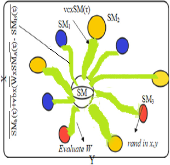
In the suggested hybridized slime mould-simulated annealing algorithm, the position vector resulting from Eqs. (8.1, 8.2, 8.3) is updated by the suggested hybrid hSMA-SA technique, and the latest location vector is adept on slime mould to compute the food sources in three stages: looming food, bind food, food grabble. The reason behind the merge of the simulated annealing technique with slime mould algorithm is to develop the actual slime mould’s exploitation phase, which has excellent global hunt ability but poor local hunt capacity. Meanwhile, it is also necessary to memorize that the simulated annealing algorithm has a strong local hunt aptitude but a weak global hunt capacity. To amalgamate SMA and SA, a heuristic strategy is chosen in which the simulated annealing method is engaged immediately successive to slime mould. Subsequently, it is noticed that the local hunt ability of traditional slime mould enhanced in the phase of exploitation in obtaining better results when blended with simulated annealing. In order to attain improvement in the suggested algorithm, the principal temperature is treated as . Here, nominates no. of attributes for the individual dataset.
The cooling itinerary for the simulated annealing method is determined using the equation presented as follows:
| 10 |
Depending on the sensitiveness in fluctuations of system energies, the temperature (T) controls the system’s state (S) evolution. ‘S’ the evolution is receptive to boorish energy variations if the value of ‘T’ is huge and if the value of ‘T’ is tiny, then ‘S’ the evolution is receptive for better energy variations. Primarily, 1.0 is the value of temperature in the beginning and it gets multiplied by a constant ‘α’ to minimize temperature (T) at the closing stages of iteration. The limit range of a constant ‘α’ is between 0.8 and 0.99. In this study, the constant ‘α’ value is picked as 0.93.
In Fig. 5, a slime mould of (X, Y) adjusts its location according to latest achieved location vectors and remains in contact with them as described in 2D and 3D views and also defines the location of the food (X*, Y*) as well as develops the search region in improvised means. Improved positions are gained by estimating the vectors and . The hSMA-SA explorative phase is same as traditional SMA. Vectors and are utilized to search globally in technical model divergence (Fig. 6). Slime mould gets expanded in the environment in search of food when vector is greater than 1 (Fig. 7). The developed hSMA-SA algorithm PSEUDO code is showcased in Figs. 8, and 9 displays the flow chart.
Fig. 5.

Probable positions in 2D and 3 D
Fig. 6.

SMA PSEUDO code
Fig. 7.

Simulated annealing algorithm PSEUDO code
Fig. 8.

PSEUDO code for hSMA-SA algorithm
Fig. 9.

Flow chart for hSMA-SA algorithm
Standard benchmark functions
The suggested hSMA-SA optimization strategy is put to the test using a cluster of distinct benchmark functions [143]. Standard benchmarks are divided into three categories: unimodal (UM), multimodal (MM), and fixed dimensions (FD). For these benchmark functions, the size, range limit, and optimal value, are determined based on objective fitness (fmin). Tables 2, 3, and 4 show the numerical formulations for UM, MM, and FD, respectively, and the findings are given in the outcomes and discussion section. The performance of typical benchmark functions is evaluated using 30 trial runs. The details of parameter setup for the proposed method are shown in Table 5.
Table 2.
Unimodal standard benchmark functions
| Functions | Dimensions | Range | fmin |
|---|---|---|---|
| 30 | [− 100, 100] | 0 | |
| 30 | [− 10,10] | 0 | |
| 30 | [− 100, 100] | 0 | |
| 30 | [− 100, 100] | 0 | |
| 30 | [− 38, 38] | 0 | |
| 30 | [− 100, 100] | 0 | |
| 30 | [− 1.28, 1.28] | 0 |
Table 3.
Multimodal standard benchmark functions
| Multimodal bench mark functions | Dim | Range | |
|---|---|---|---|
| 30 | [− 500, 500] | − 418.98295 | |
| 30 | [− 5.12, 5.12] | 0 | |
| 30 | [− 32, 32] | 0 | |
| 30 | [− 600, 600] | 0 | |
|
where
|
30 | [− 50, 50] | 0 |
| 30 | [− 50, 50] | 0 |
Table 4.
Fixed-dimension benchmark functions
| Fixed-dimension (FD) benchmark functions | Dimension | Range | |
|---|---|---|---|
| 2 | [− 65.536, 65.536] | 1 | |
| 4 | [− 5, 5] | 0.00030 | |
| 2 | [− 5, 5] | − 1.0316 | |
| 2 | [− 5, 5] | 0.398 | |
| 2 | [− 2,2] | 3 | |
| 3 | [1, 3] | − 3.32 | |
| 6 | [0, 1] | − 3.32 | |
| 4 | [0,10] | − 10.1532 | |
| 4 | [0, 10] | − 10.4028 | |
| 4 | [0, 10] | − 10.5363 |
Table 5.
Parameter constraints for the suggested technique
| Parameter setting | hSMA-SA |
|---|---|
| Search agents | 30 |
| Count of iterations for benchmark problems (unimodal, multimodal and fixed dimension) | 500 |
| Count of iterations for engineering optimal designs | 500 |
| Count of trial runs for each function and engineering optimal designs | 30 |
Thirty search agents are used to go through the entire research, with a maximum of 500 iterations. The proposed hSMA-SA was evaluated using the MATLAB R2016a program using a laptop of Intel corei3 processor with an 8 GB RAM and 7th generation CPU.
According to the results of the comparative study, the suggested heuristic technique significantly boosts the rate of convergence as well as develops its capacity to quickly run away from local area stagnation.
Results and analysis
The offered slime mould-simulated annealing method is assessed on three primary modules of customary benchmark functions in this study effort to validate the success rate of the suggested hSMA-SA technique. The exploitation and convergence rate of hSMA-SA are assessed using unimodal benchmark functions with a single optimal solution. As the name indicates, multimodal replicates several perfect solutions, as a result, these can be used to check for exploration and prevent finding a local optimal solution. The distinction among multimodal and fixed-dimension benchmark functions determines the design variables. These design variables will be saved in fixed-dimension benchmark functions, which will uphold a graphic representation of preceding search space data to compare with multimodal functions.
For detailed study, a documentation of the outcomes for the launched hSMA-SA technique was supplied; in the table form indicating statistical outputs, time of computation, and evaluation of the technique by executing with 500 iterations and 30 runs.
Evaluation of unimodal functions (exploitation)
The search progress for the finest place stands upon the potential of search agents to arrive nearer to source. At the time of the search procedure, there is a chance for various agents to get ensnare far or nearby in view of the phases exploration and exploitation. Exploration falls below global search whereas exploitation refers to local search. The results of unimodal functions have a statistical analysis in selected points such as search record, convergence behavior, average fitness of population. The search record in the trail runs graph shows the locations of slime mould. The graph of convergence explains the variation in the position of slime mould during optimization procedure. The average fitness of the population describes the variations in the average population during whole optimization procedure. This better convergence certifies the effectiveness of the suggested algorithm. The low p value shown in Table 9, which was acquired using the statistical Wilcoxon rank sum test and t test to examine the proposed algorithm’s detailed behavior, indicates that the produced algorithm has better convergence and is more effective. At a 95% level of significance, the h value further supports the null hypothesis. The suggested algorithm’s parametric test demonstrates that the null hypothesis is rejected at the alpha significance level. If h = 1, the null hypothesis has been rejected at the alpha significance level. If h = 0, the null hypothesis was not successfully rejected at the alpha significance level.
Table 9.
Test results for multimodal functions using hSMA-SA technique
| Function | Mean | Standard deviation | Best fitness value | Worst fitness value | Median | Wilcoxon rank sum test | t test | |
|---|---|---|---|---|---|---|---|---|
| p value | p value | h value | ||||||
| Schwefel sine function (F8) | − 12,569.02623 | 0.43623993 | − 12,569.48529 | − 12,567.9831 | − 12,569.15434 | 1.73E−06 | 4.22E−131 | 1 |
| Rastrigin function (F9) | 0 | 0 | 0 | 0 | 0 | 1 | 0 | 1 |
| The Ackley function (F10) | 8.88E−16 | 0 | 8.88E−16 | 8.88E−16 | 8.88E−16 | 4.32E−08 | 0 | 1 |
| Penalized penalty#1 function (F12) | 0.012678845 | 0.012483005 | 9.69E−05 | 0.039727727 | 0.007266933 | 1.73E−06 | 5.31E−06 | 1 |
| Levi N. 13 function (F13) | 0.002689783 | 0.001733379 | 0.000388677 | 0.007871366 | 0.002737656 | 1.73E−06 | 2.30E−09 | 1 |
Figure 10 showcases the characteristic curves of unimodal benchmark functions and Fig. 11 shows a comparison of hSMA-SA with other different algorithms. It is observed from the curves of convergence of proposed algorithm converges to optimum very soon. To ensure the aptness of the launched technique, every test function is assumed with SMA and SA. The statistical outputs in Table 6 exhibit the unimodal functions in view of mean, standard deviation, best fitness value, worst fitness, median, p value and t value. There are a few areas of global optima and a few areas get jammed in local optima in search region. The global search procedure finds the exploration phase while the local search procedure explores the exploitation. The appraisal of any technique is inspected by its capability in attaining maxima or minima within a little time of computation. Table 7 displays the time of computation in view of best, average as well as worst time. Table 8 displays the evaluation of hSMA-SA technique with other already available methods such as LSA [144], (SCA) [102], BRO [145], DA [146], OEGWO [147], MFO [34], PSA [74], HHO-PS [50], (SSA) [148], SHO [46], GWO [149], HHO [78], MVO [24], ECSA [150], PSO [151], TSO [109], ALO [152], and LF-SMA [8] considering standard deviation and average value. There is a variation in benchmark functions in view of characteristics. All these functions differ in their search abilities in the zones of exploration and exploitation. In this context, test judgment for six unimodal benchmark functions is examined. The test results for each function are reported in terms of average and standard deviation after 30 trial runs and 500 iterations. To examine the influence of SA on the solutions of hSMA-SA the scalability measurement is conceded. Table 8 displaying the statistical result announces a significant gap between hSMA-SA and other techniques. It is clear from Table 8 that by injecting SA technique, the SMA gained strength to enhance exploration and exploitation phases. The results of hSMA-SA when compared with SCA, ALO, PSA, SSA, MVO, BRO, PSO, MFO, DA, and GWO show noteworthy feat in handling with F3, F5, and F6 test functions in terms of standard deviation and average value. According to Fig. 11 convergence curves, it is noticed that with enhanced efficacy, the optimality results shoot up. The former approaches shown converge early. Moreover, to prove the success of the introduced method, every benchmark function’s independent trial runs are shown in Fig. 12. By comparison, it is proved that the SA algorithm promotes to investigate the local search phase with high intensity.
Fig. 10.

3D view of unimodal functions
Fig. 11.

Convergence curve of hSMA-SA with known algorithms for F1–F6 functions
Table 6.
Test note for unimodal functions using hSMA-SA technique
| Function | Mean | Standard deviation | Best fitness value | Worst fitness value | Median | Wilcoxon rank sum test | t test | |
|---|---|---|---|---|---|---|---|---|
| p value | p value | h value | ||||||
| Sphere function (F1) | 1.4E−300 | 0 | 0 | 4.2059E−299 | 0 | 0.125 | 0 | 1 |
| Schwefel absolute function (F2) | 1.9E−159 | 1.0209E−158 | 0 | 5.5926E−158 | 4.6226E−200 | 1.7344E−06 | 0.32386916 | 0 |
| Schwefel double sum function (F3) | 6.1E−121 | 3.309E−120 | 0 | 1.8126E−119 | 2.5788E−151 | 2.56308E−06 | 0.324043719 | 0 |
| Schwefel max. function (F4) | 3.6E−163 | 2.2228E−162 | 1.0007E−262 | 1.088E−161 | 4.4998E−199 | 1.7344E−06 | 0.378435872 | 0 |
| Rosenbrock function (F5) | 11.77822 | 12.89147042 | 0.011463167 | 28.35510393 | 3.286513444 | 1.7344E−06 | 2.50694E−05 | 1 |
| The step function (F6) | 0.007059 | 0.004749705 | 0.001719961 | 0.021628358 | 0.005572663 | 1.73E−06 | 5.63E−09 | 1 |
Table 7.
Time for execution for unimodal functions using hSMA-SA technique
| Function | Best time | Average time | Worst time |
|---|---|---|---|
| Sphere function (F1) | 190.3906 | 219.1385417 | 297.39063 |
| Schwefel absolute function (F2) | 122.7188 | 133.9958333 | 155.51563 |
| Schwefel double sum function (F3) | 137.2188 | 144.546875 | 162.70313 |
| Schwefel max. function (F4) | 111.875 | 176.4671875 | 307.20313 |
| Rosenbrock function (F5) | 90.25 | 112.4067708 | 150.95313 |
| The step function (F6) | 195.25 | 212.9197917 | 327.8125 |
Table 8.
Evaluation for unimodal problems
| Algorithm | Parameters | Unimodal Benchmark functions | |||||
|---|---|---|---|---|---|---|---|
| sphere function (F1) | Schwefel absolute function (F2) | Schwefel double sum function (F3) | Schwefel max. function (F4) | Rosenbrock function (F5) | The step function (F6) | ||
| Lightning search algorithm (LSA) [144] | Avg | 4.81067E−08 | 3.340000000 | 0.024079674 | 0.036806544 | 43.24080402 | 1.493275733 |
| S. deviation | 3.40126E−07 | 2.086007800 | 0.005726198 | 0.156233023 | 29.92194448 | 1.302827039 | |
| Dragonfly algorithm (DA) [146] | Avg | 2.850E−19 | 1.490E−06 | 1.290E−07 | 9.88E−04 | 7.6 | 4.170E−17 |
| S. deviation | 7.160E−19 | 3.760E−06 | 2.100E−07 | 2.78E−03 | 6.79 | 1.320E−16 | |
| Battle Royale optimization algorithm (BRO) [145] | Avg | 3.0353E−09 | 0.000046 | 54.865255 | 0.518757 | 99.936848 | 2.8731E−08 |
| S. deviation | 4.1348E−09 | 0.000024 | 16.117329 | 0.403657 | 82.862958 | 1.8423E−08 | |
| Multi-verse optimizer (MVO) [24] | Avg | 2.08583 | 15.9247 | 453.200 | 3.12301 | 1272.13 | 2.29495 |
| S. deviation | 0.64865 | 44.7459 | 177.0973 | 1.58291 | 1479.47 | 0.63081 | |
| Opposition-based enhanced grey wolf optimization algorithm (OEGWO) [147] | Avg | 2.49 × 10⁻³⁴ | 4.90 × 10⁻²⁵ | 1.01 × 10⁻¹ | 1.90 × 10⁻⁵ | 2.72 × 101 | 1.40 × 1000 |
| S. deviation | 7.90 × 10⁻³⁴ | 6.63 × 10⁻²⁵ | 3.21 × 10⁻¹ | 2.43 × 10⁻⁵ | 7.85 × 101 | 4.91 × 10⁻¹ | |
| Particle swarm optimization (PSO) [151] | Avg | 1.3E−04 | 0.04214 | 7.01256E+01 | 1.08648 | 96.7183 | 0.00010 |
| S. deviation | 0.0002.0E−04 | 0.04542 | 2.1192E+01 | 3.1703E+01 | 6.01155E+01 | 8.28E−05 | |
| Photon search algorithm (PSA) [74] | Avg | 15.3222 | 2.2314 | 3978.0837 | 1.1947 | 332.6410 | 19.8667 |
| S. deviation | 27.3389 | 1.5088 | 3718.9156 | 1.0316 | 705.1589 | 33.4589 | |
| Sine–cosine algorithm (SCA) [102] | Avg | 0.000 | 0.000 | 0.0371 | 0.0965 | 0.0005 | 0.0002 |
| S. deviation | 0.000 | 0.0001 | 0.1372 | 0.5823 | 0.0017 | 0.0001 | |
| Hybrid Harris hawks optimizer–pattern search algorithm (hHHO-PS) [50] | Avg | 9.2 × 10–017 | 8.31E | 5.03 × 10⁻²⁰ | 6.20 × 10–54 | 2.18 × 10⁻⁹ | 3.95 × 10⁻¹⁴ |
| S. deviation | 5E−106 | 4.46 × 10–53 | 1.12 × 10⁻¹⁹ | 1.75 × 10–53 | 6.38 × 10⁻¹⁰ | 3.61 × 10⁻¹⁴ | |
| Ant lion optimizer (ALO) [152] | Avg | 2.59E−10 | 1.84E−06 | 6.07E−10 | 1.36E−08 | 0.3467724 | 2.56E−10 |
| S. deviation | 1.65E−10 | 6.58E−07 | 6.34E−10 | 1.81E−09 | 0.10958 | 1.09E−10 | |
| Spotted hyena optimizer (SHO) [46] | Avg | 0 | 0 | 0 | 7.78E−12 | 8.59E+00 | 2.46E−01 |
| S. deviation | 0 | 0 | 0 | 8.96E−12 | 5.53E−01 | 1.78E−01 | |
| Moth flame optimizer (MFO) [34] | Avg | 0.00011 | 0.00063 | 696.730 | 70.6864 | 139.1487 | 0.000113 |
| S. deviation | 0.00015 | 0.00087 | 188.527 | 5.27505 | 120.2607 | 9.87E−05 | |
| Harris hawks optimizer (HHO) [78] | Avg | 1.06 × 10–90 | 6.92 × 10–51 | 1.25 × 10–80 | 4.46 × 10–48 | 0.015002 | 0.000115 |
| S. deviation | 5.82 × 10–90 | 2.47 × 10–50 | 6.63 × 10–80 | 1.70 × 10–47 | 0.023473 | 0.000154 | |
| Grey wolf optimizer (GWO) [149] | Avg | 6.590E−29 | 7.180E−18 | 3.20E−−07 | 5.610E−08 | 26.8125 | 0.81657 |
| S. deviation | 6.3400E−07 | 0.02901 | 7.9.1495E+01 | 1.31508 | 69.9049 | 0.00012 | |
| Enhanced crow search algorithm (ECSA) [150] | Avg | 7.4323E−119 | 5.22838E−59 | 3.194E−102 | 3.04708E−52 | 7.996457081 | 0.400119079 |
| S. deviation | 4.2695E−118 | 2.86361E−58 | 1.7494E−101 | 1.66895E−51 | 0.661378213 | 0.193939866 | |
| Salp swarm algorithm (SSA) [148] | Avg | 0.000 | 0.2272 | 0.000 | 0.000 | 0.000 | 0.000 |
| S. deviation | 0.000 | 1.000 | 0.000 | 0.6556 | 0.000 | 0.000 | |
| Transient search optimization (TSO) [109] | Avg | 1.18 × 10–99 | 8.44 × 10–59 | 3.45 × 1041 | 1.28E−53 | 8.10 × 10⁻² | 3.35 × 10⁻³ |
| S. deviation | 6.44 × 10–99 | 3.93 × 10–58 | 1.26 × 10–41 | 6.58 × 10–53 | 11 | 6.82 × 10⁻³ | |
| LF-SMA [8] | Avg | 1.58E−156 | 2.74E−171 | 5.2412 | 0.0006 | 5.90E−05 | 0.0008 |
| S. deviation | 7.53E−156 | 0 | 10.229 | 0.0002 | 6.38E−05 | 0.0008 | |
| Proposed algorithm hSMA-SA | Avg | 1.4E−300 | 1.9E−159 | 6.1E−121 | 3.6E−163 | 11.77822 | 0.007059 |
| S. deviation | 0 | 1.0209E−158 | 3.309E−120 | 2.2228E−162 | 12.89147042 | 0.004749705 | |
Fig. 12.

Trial runs of SMA and hSMA-SA for F1–F6 functions
Evaluation of a few multimodal functions (exploration)
Figure 13 showcases the characteristic curves of multimodal benchmark functions and Fig. 14 presents comparison between hSMA-SA and other techniques. In this study, F8, F9, F10, F12, and F13 multimodal benchmark functions are examined considering 30 trial runs with 500 iterations and the results are tabulated in Table 9. The execution time for the simulation process for multimodal are recorded and tabled in Table 10. Table 11 contains the information of compared results of hSMA-SA algorithm with other already available metaheuristic search algorithms such as LSA [144], (SCA) [102], BRO [145], DA [146], OEGWO [147], MFO [34], PSA [74], HHO-PS [50], (SSA) [148], SHO [46], GWO [149], HHO [78], MVO [24], ECSA [150], PSO [151], TSO [109], ALO [152], and LF-SMA [8] considering standard deviation and average value. The results of multimodal functions have a statistical analysis in selected points such as search record, convergence behavior, and average fitness of population. The search record in the trail runs graph shows the positions of slime mould. The graph of convergence explains the variation in the position of slime mould during optimization procedure. The average fitness of the population describes the changes in the average population during whole optimization procedure. This better convergence certifies the effectiveness of the suggested algorithm. The created algorithm has better convergence and is more efficient, according to the low p value supplied in Table 9, which was obtained using the statistical Wilcoxon rank sum test and t test to check the recommended algorithm’s detailed behavior. The h value further validates the null hypothesis at a 95% level of significance. The null hypothesis is rejected at the alpha significance level by the parametric test of the provided method. At the alpha significance level, the null hypothesis has been rejected if h = 1. If h = 0, the alpha significance threshold did not allow for a valid rejection of the null hypothesis. It is noted from Fig. 14 that the results of F8, F9, F10, F12, and F13 multimodal benchmark functions have improved convergence curves using hSMA-SA, justifying the aptness of the algorithm in verdict solutions for the multimodal functions. Table 11 shows the analysis of statistical data revealing that the optimality of multimodal benchmark functions is slightly gained better results by applying SA algorithm. The average and standard deviation outcomes reveal that hSMA-SA performs better for all selected five test functions than ECSA, HHO-PS, and LSA. It is recorded from the convergence curves of Fig. 14 that hSMA-SA allows optimal convergences for a few test functions. From the comparison of convergence, it is well understood that hSMA-SA converges soon and catches the run as early as it attains the end condition. From the comparative curves of Fig. 14, it is noticeable that the proposed technique acts good in handling F9, F10, and F13 and performs comparatively better than F8 and F12. Moreover, to prove the success of the proposed technique, every benchmark function’s independent trial runs are shown in Fig. 15. The comparison study proved that hSMA-SA algorithm appreciably searches with extra intensity in the local and global search space.
Fig. 13.

3D view of multimodal standard benchmark functions
Fig. 14.

Convergence curve of hSMA-SA with known algorithms for multimodal functions
Table 10.
Time of execution for multimodal functions via hSMA-SA technique
| Function | Best time | Average time | Worst time |
|---|---|---|---|
| Schwefel sine function (F8) | 659.2031 | 666.775 | 686.51563 |
| Rastrigin function (F9) | 513.2031 | 532.9604167 | 586.29688 |
| The Ackley function (F10) | 566.0469 | 575.2671875 | 599.53125 |
| Penalized penalty#1 function (F12) | 2008.016 | 2101.541146 | 2290.125 |
| Levi N. 13 function (F13) | 2062.094 | 2145.145313 | 2304.7031 |
Table 11.
Comparison for multimodal benchmark functions
| Algorithm | Parameters | Multimodal benchmark functions | ||||
|---|---|---|---|---|---|---|
| Schwefel sine function (F8) | Rastrigin function (F9) | The Ackley function (F10) | Penalized penalty#1 function (F12) | Levi N. 13 function (F13) | ||
| Lightning search algorithm (LSA) [144] | Avg | − 8001.3887 | 62.7618960 | 1.077446947 | 2.686199995 | 0.007241875 |
| St. deviation | 669.159310 | 14.9153021 | 0.337979509 | 0.910802774 | 0.006753356 | |
| Dragonfly algorithm (DA) [146] | Avg | − 2.860E+03 | 1.600E+01 | 2.310E−01 | 3.110E−02 | 2.200E−03 |
| St. deviation | 3.840E+02 | 9.480E+00 | 4.870E−01 | 9.830E−02 | 4.630E−03 | |
| Battle Royale optimization algorithm (BRO) [145] | Avg | − 7035.2107 | 48.275350 | 0.350724 | 0.369497 | 0.000004 |
| St. deviation | 712.33269 | 14.094585 | 0.688702 | 0.601450 | 0.000020 | |
| Multi-verse optimizer (MVO) [24] | Avg | − 1.170E+04 | 1.180E+02 | 4.070E+00 | 2.460E+00 | 2.200E−01 |
| St. deviation | 9.370E+02 | 3.930E+01 | 5.500E+00 | 7.900E−01 | 9.000E−02 | |
| Opposition-based enhanced grey wolf optimization algorithm (OEGWO) [147] | Avg | − 3.36 × 10³ | 8.48 × 10⁻¹ | 9.41 × 10⁻¹⁵ | 9.36 × 10–02 | 1.24E+00 |
| St. deviation | 3.53 × 10² | 4.65E+00 | 3.56 × 10⁻¹⁵ | 3.95 × 10–02 | 2.09 × 10⁻¹ | |
| Particle swarm optimization (PSO) [151] | Avg | − 4.8400E+04 | 4.670E+01 | 2.760E−01 | 6.9200E−04 | 6.6800E−04 |
| St. deviation | 1.1500E+04 | 1.160E+01 | 5.090E−01 | 2.6300E−03 | 8.9100E−04 | |
| Photon search algorithm (PSA) [74] | Avg | 11,648.5512 | 7.3763 | 1.6766 | 0.1716 | 1.5458 |
| St. deviation | 1230.4314 | 9.1989 | 0.9929 | 0.2706 | 3.3136 | |
| Sine–cosine algorithm (SCA) [102] | Avg | 1.000E+00 | 0.000E+00 | 3.800E−01 | 0.000E+00 | 0.000E+00 |
| St. deviation | 3.600E−03 | 7.300E−01 | 1.000E+00 | 0.000E+00 | 0.000E+00 | |
| Hybrid Harris hawks optimizer–pattern search algorithm (hHHO-PS) [50] | Avg | − 12,332 | 00 | 8.88 × 10⁻⁶ | 2.94 × 10⁻¹⁵ | 1.16 × 10⁻¹³ |
| St. deviation | 335.7988 | 0 | 0 | 3.52E−15 | 1.15E−13 | |
| Ant lion optimizer (ALO) [152] | Avg | − 1.61E+03 | 7.71E−06 | 3.73E−15 | 9.75E−12 | 2.00E−11 |
| St. deviation | 3.14E+02 | 8.45E−06 | 1.50E−15 | 9.33E−12 | 1.13E−11 | |
| Spotted hyena optimizer (SHO) [46] | Avg | − 1.16E × 103 | 0.00E+00 | 2.48E+000 | 3.68 × 10⁻² | 9.29 × 10⁻¹ |
| St. deviation | 2.72E × 102 | 0.00E+00 | 1.41E+000 | 1.15 × 10⁻² | 9.52 × 10⁻² | |
| Moth flame optimizer (MFO) [34] | Avg | − 8.500E+03 | 8.460E+01 | 1.260E+00 | 8.940E−01 | 1.160E−01 |
| St. deviation | 7.260E+02 | 1.620E+01 | 7.300E−01 | 8.810E−01 | 1.930E−01 | |
| Harris hawks optimizer (HHO) [78] | Avg | − 12,561.38 | 0 | 8.88 × 10⁻¹⁶ | 8.92 × 10⁻⁶ | 0.000101 |
| St. deviation | 40.82419 | 0 | 0 | 1.16 × 10⁻⁵ | 0.000132 | |
| Grey wolf optimizer (GWO) [149] | Avg | − 6.1200E+02 | 3.1100E−02 | 1.0600E−14 | 5.3400E−03 | 6.5400E−02 |
| St. deviation | − 4.0900E+02 | 4.740E+01 | 7.7800E−03 | 2.0700E−03 | 4.470E−03 | |
| Enhanced crow search algorithm (ECSA) [150] | Avg | − 2332.3867 | 0 | 8.88178E−16 | 0.11738407 | 0.444690657 |
| St. deviation | 223.93995 | 0 | 0 | 0.2849633 | 0.199081675 | |
| Salp swarm algorithm (SSA) [148] | Avg | 5.570E−02 | 0.000E+00 | 1.950E−01 | 1.420E−01 | 8.320E−02 |
| St. deviation | 8.090E−01 | 0.000E+00 | 1.530E−01 | 5.570E−01 | 7.060E−01 | |
| Transient search optimization (TSO) [109] | Avg | − 12,569.5 | 00 | 8.88 × 10⁻¹⁶ | 1.30 × 10⁻⁴ | 7.55 × 10⁻⁴ |
| St. deviation | 1.81 × 10⁻² | 00 | 0 | 1.67 × 10⁻⁴ | 1.74 × 10⁻³ | |
| LF-SMA [8] | Avg | 0.0004 | − 3.2865 | − 17.363 | 0.0130 | 1.07E−12 |
| St. deviation | 5.89E−05 | 0.0536 | 2.1907 | 0.0090 | 2.29E−12 | |
| Proposed algorithm hSMA-SA | Avg | − 12,569.02623 | 0 | 8.88E−16 | 0.012678845 | 0.002689783 |
| St. deviation | 0.43623993 | 0 | 0 | 0.012483005 | 0.001733379 | |
Fig. 15.

Trial runs of SMA and hSMA-SA for multimodal benchmark functions
Evaluation of a few fixed-dimension functions
Figure 16 presents the characteristic curves of fixed-dimension functions and Fig. 17 showcases the comparison between hSMA-SA and other techniques. In this article, F15, F16, F17, F18, and F23 fixed-dimension benchmark functions are examined considering 30 trial runs with 500 iterations and the results are shown in Fig. 18. Using hSMA-SA, the simulation results for fixed-dimension functions are recorded in Table 12. The execution time for simulation process for fixed-dimension functions are recorded and tabled in Table 13. Table 14 contains the information of compared results of hSMA-SA algorithm with other already available metaheuristic search algorithms such as LSA [144], (SCA) [102], MFO [34], PSA [74], HHO-PS [50], (SSA) [148], SHO [46], GWO [149], HHO [78], MVO [24], ECSA [150], PSO [151], TSO [109], and ALO [152] considering standard deviation and average value. The results of fixed-dimension functions have a statistical analysis in selected points such as search record, convergence behavior, average fitness of population. The search record in the trail runs graph shows the positions of slime mould. The graph of convergence explains the variation in the location of slime mould during optimization procedure. The average fitness of the population describes the changes in the average population during whole optimization procedure. This better convergence certifies the effectiveness of the suggested algorithm. The statistical Wilcoxon rank sum test and t test were also used to confirm the suggested algorithm’s detailed behavior, and the low p value provided in Table 12 indicates that the produced algorithm has better convergence and is more effective. In addition, the null hypothesis is validated at a 95% level of significance by the h value. The parametric test of the suggested technique rejects the null hypothesis at the alpha significance level. If h = 1, the null hypothesis has been rejected at the alpha significance level. The alpha significance criterion did not permit a legitimate rejection of the null hypothesis if h = 0. It is noted from Fig. 17 that the results of F15, F16, F17, F18, and F23 fixed-dimension benchmark functions have improved convergence curves using hSMA-SA, justifying the aptness of the algorithm in verdict solutions for the fixed dimensions. The average and standard deviation outcomes reveal that hSMA-SA performs better for all five test functions than GWO, HHO-PS, SCA, PSO. It can be recorded from the convergence curves of Fig. 17 that hSMA-SA allows optimal convergences for a few test functions. From the comparison of convergence, it is well understood that hSMA-SA converges soon and catches the run as early as it attains the end condition. From the comparative curves of Fig. 17, it is noticeable that the proposed technique acts good in handling with F15, F16, and F23 and performs better than F17 and F18. Figure 18 reveals that the trial runs of the proposed hSMA-SA algorithm notably search in local and global space to find the optimal solution.
Fig. 16.

Fixed-dimension benchmark functions in 3D
Fig. 17.

Convergence curve of hSMA-SA with known algorithms for fixed-dimension functions
Fig. 18.

Trial runs of SMA and hSMA-SA for fixed-dimension functions
Table 12.
Test outcomes of fixed-dimension functions using hSMA-SA technique
| Function | Mean | Standard deviation | Best fitness value | Worst fitness value | Median | Wilcoxon rank sum test | t test | |
|---|---|---|---|---|---|---|---|---|
| p value | p value | h value | ||||||
| Brad function (F15) | 0.00057313 | 0.000284537 | 0.000308341 | 0.001243214 | 0.000443492 | 1.7344E−06 | 6.78516E−12 | 1 |
| Camel function—six hump (F16) | − 1.031628453 | 5.42E−10 | − 1.031628453 | − 1.031628451 | − 1.031628453 | 1.73E−06 | 7.16E−271 | 1 |
| Branin RCOS function (F17) | 0.397887411 | 8.70E−08 | 0.397887358 | 0.397887735 | 0.397887381 | 1.73E−06 | 6.34E−195 | 1 |
| Goldstein-price function (F18) | 3 | 2.77E−11 | 3 | 3 | 3 | 1.73E−06 | 0 | 1 |
| Hybrid composition function #3 (F23) | − 8.732008933 | 3.082499131 | − 10.52915056 | − 5.172702813 | − 10.49417343 | 0.25 | 0.039117859 | 1 |
Table 13.
Execution time of fixed-dimension functions using hSMA-SA technique
| Function | Best time | Average time | Worst time |
|---|---|---|---|
| Brad function (F15) | 53.20313 | 56.91614583 | 65.640625 |
| Camel function—six hump (F16) | 43.98438 | 46.20729167 | 51.90625 |
| Branin RCOS function (F17) | 42.40625 | 44.60052083 | 47.453125 |
| Goldstein-price function (F18) | 20.79688 | 21.53385417 | 22.5625 |
| Hybrid composition function #3 (F23) | 0.078125 | 0.229166667 | 0.484375 |
Table 14.
Benchmark functions with fixed dimensions compared with other techniques
| Algorithm | Parameters | Fixed-dimension benchmark functions | ||||
|---|---|---|---|---|---|---|
| Brad function (F15) | Camel function—six hump (F16) | Branin RCOS function (F17) | Goldstein-price function (F18) | Hybrid composition function #3 (F23) | ||
| Lightning search algorithm (LSA) [144] | Mean | 0.024148546 | 0.000534843 | − 1.031628453 | 3.000000000 | − 7.910438367 |
| St. deviation | 0.047279168 | 0.000424113 | 0.000000000 | 3.34499E−15 | 3.596042666 | |
| Enhanced crow search algorithm (ECSA) [150] | Mean | 0.000327 | − 1.03161 | 0.397993 | 3.00003 | − 10.5359 |
| St. deviation | 1.24337E−05 | 2.20378E−05 | 1.16E−04 | 2.752E−05 | 4.62E−04 | |
| Salp swarm algorithm (SSA) [148] | Mean | 0.0000 | 0.1952 | 0.0000 | 0.1417 | N/A |
| St. deviation | 0.0000 | 0.1527 | 0.0651 | 0.5571 | N/A | |
| Multi-verse optimizer (MVO) [24] | Mean | 30.00705 | 50.00061 | 190.3 | 160.5312 | N/A |
| St. deviation | 48.30615 | 52.70461 | 128.6659 | 158.2887 | N/A | |
| Transient search optimization (TSO) [109] | Mean | 9.01 × 10⁻⁴ | − 1.06 × 10⁻¹ | 3.97 × 10⁻¹ | 3.00E+000 | 10.5267 |
| St. deviation | 1.06 × 10⁻⁴ | 2.86 × 10⁻¹¹ | 2.46 × 10⁻¹ | 9.05E+000 | 2.63 × 10⁻² | |
| Particle swarm optimization (PSO) [151] | Mean | 0.4081 | 0.6181 | 0.4694 | 0.3566 | N/A |
| St. deviation | 0.8317 | 0.5347 | 0.8406 | 0.7841 | N/A | |
| Photon search algorithm (PSA) [74] | Mean | 0.0077 | − 1.036 | 0.3979 | 3 | − 9.8189 |
| St. deviation | 0.0224 | 2.33 × 10⁻⁷ | 1.41 × 10⁻⁷ | 1.36 × 10⁻⁵ | 1.8027 | |
| Sine–cosine algorithm (SCA) [102] | Mean | 0.0230 | 0.0497 | 0.0000 | 0.0129 | N/A |
| St. deviation | 0.0676 | 0.4921 | 0.1105 | 0.0134 | N/A | |
| Hybrid Harris hawks optimizer–pattern search algorithm (hHHO-PS) [50] | Mean | 0.000307 | − 1.03163 | 0.397887 | 3 | − 10.5364 |
| St. deviation | 1.65 × 10⁻¹³ | 1.11 × 10⁻¹⁶ | 00 | 2.63 × 10⁻¹⁵ | 7.69 × 10⁻¹⁵ | |
| Ant lion optimizer (ALO) [152] | Mean | 14.56498 | 175.1532 | 316.0686 | 4.399206 | N/A |
| St. deviation | 32.22876 | 46.50001 | 13.02047 | 1.66107 | N/A | |
| Spotted hyena optimizer (SHO) [46] | Mean | 2.70 × 10⁻³ | − 1.0316 | 0.398 | 3.000 | − 1.68E+000 |
| St. deviation | 5.43 × 10⁻³ | 5.78 × 10⁻¹⁴ | 1.26 × 10⁻¹⁴ | 2.66 × 10⁻¹³ | 2.64 × 10⁻¹ | |
| Moth flame optimizer (MFO) [34] | Mean | 66.73272 | 119.0146 | 345.4688 | 10.4086 | N/A |
| St. deviation | 53.22555 | 28.3318 | 43.11578 | 3.747669 | N/A | |
| Harris hawks optimizer (HHO) [78] | Mean | 0.00035 | − 1.03163 | 0.397895 | 3.000001225 | − 5.78398 |
| St. deviation | 3.20 × 10⁻⁵ | 1.86 × 10⁻⁹ | 1.60 × 10⁻⁵ | 4.94 × 10⁻⁶ | 1.712458 | |
| Grey wolf optimizer (GWO) [149] | Mean | 0.000337 | − 1.03163 | 0.397889 | 3.000028 | − 10.5343 |
| St. deviation | 0.000625 | − 1.03163 | 0.397887 | 3 | − 8.55899 | |
| hSMA-SA-proposed algorithm | Mean | 0.00057313 | − 1.031628453 | 0.397887411 | 3 | − 8.732008933 |
| St. deviation | 0.000284537 | 5.42E−10 | 8.70E−08 | 2.77E−11 | 3.082499131 | |
Thus, the outcomes for all benchmark functions are framed in Tables 6, 7, 8, 9, 10, 11, 12, 13, and 14 and the assessment of proposed hSMA-SA algorithm convergence curves for all benchmark functions are shown in Figs. 11, 14 and 17, and trial runs for all functions are depicted in Figs. 12, 15, and 18. The above result clearly shows that the proposed hSMA-SA algorithm is better than other algorithms. It also proves that hSMA-SA has proficient performance and very good convergence capability. As per the experiments carried out, the proposed hSMA-SA algorithm has given better results which can have balance between exploration and exploitation.
Engineering-based optimization design problems
Eleven types of engineering-based optimization schemes are investigated to vote the usefulness of the recommended hSMA-SA algorithm. The hSMA-SA method is used to tackle these issues. As shown in Fig. 30, the findings for engineering design challenges were explored utilizing multiple metaheuristic search methods, with convergence curves compared to the classic SMA approach. Table 15 lists the engineering design problems, while Table 16 lists the fitness, average values, median values, standard deviation, as well as worst fitness values. Table 17 lists the Wilcoxon Rank sum test and t test values, while Table 18 lists the time of computation for engineering design issues.
Fig. 30.


Convergence curve and trial run for special engineering functions with SMA and hSMA-SA
Table 15.
Special engineering designs
| Special engineering function | I beam | Multiple disk clutch brake | Rolling element bearing | Spring design | Gear train | Speed reducer | Cantilever Beam | Three-bar truss | Pressure vessel | Welded beam | Belleville spring |
|---|---|---|---|---|---|---|---|---|---|---|---|
| Key objective | Minimize vertical deflection | Minimize weight | Maximize dynamic load | Minimize weight | Minimize gear ratio | Minimize weight | Minimize weight | Minimize weight | Minimize cost | Minimize cost | Minimize weight |
| Count of discrete variables | 4 | 5 | 10 | 3 | 4 | 7 | 5 | - | 4 | 4 | - |
| Count of constraint | 4 | 8 | 9 | 4 | 1 | 11 | 1 | 3 | 4 | 7 | 5 |
Table 16.
hSMA-SA outcomes of special engineering design problems
| Name of design | Mean | Standard deviation | Best | Worst | Median |
|---|---|---|---|---|---|
| Spring design | 0.013756625 | 0.001561454 | 0.012715329 | 0.017730689 | 0.012792095 |
| Pressure vessel | 6182.99867 | 451.5409611 | 5885.788679 | 7318.734233 | 5959.213246 |
| Multiple disk clutch brake (discrete variables) | 0.394509836 | 0.006702453 | 0.389654341 | 0.404666132 | 0.389665239 |
| I beam design | 0.00662596 | 3.62923E–09 | 0.006625958 | 0.006625976 | 0.006625959 |
| Speed reducer problem | 2994.491782 | 0.023016734 | 2994.474041 | 2994.595766 | 2994.486745 |
| Cantilever beam design | 1.303678864 | 0.000374902 | 1.303294886 | 1.305199129 | 1.303629652 |
| Three-bar truss problem | 270.2539599 | 2.361580897 | 264.2694671 | 273.4690636 | 270.9094455 |
| Welded beam | 1.778021239 | 0.143521546 | 1.725134404 | 2.321842966 | 1.728195083 |
| Gear train | 2.70E−11 | 7.34E−11 | 4.13E−16 | 3.10E−10 | 1.79E−12 |
| Belleville spring | 6.44E+22 | 7.81E+22 | 5.251751783 | 3.78E+23 | 5.69E+22 |
| Rolling element bearing | − 85,525.79232 | 36.27683994 | − 85,539.05618 | − 85,346.80626 | − 85,538.4479 |
Table 17.
Parametric test outcomes using proposed hSMA-SA technique
| Name of design | p value | t value | h value |
|---|---|---|---|
| Belleville spring | 1.72E−06 | 9.71E−05 | 1 |
| Pressure vessel | 1.73E−06 | 9.20E−35 | 1 |
| Spring design | 1.73E−06 | 2.98E−29 | 1 |
| I beam design | 1.7344E−06 | 2.3546E−183 | 1 |
| Multiple disk clutch brake (discrete variables) | 1.73E−06 | 4.24E−53 | 1 |
| Three-bar truss problem | 1.73E−06 | 1.80E−61 | 1 |
| Speed reducer problem | 1.73E−06 | 4.36E−150 | 1 |
| Rolling element bearing | 1.73E−06 | 1.42E−99 | 1 |
| Cantilever beam design | 1.73E−06 | 1.81E−104 | 1 |
| Gear train | 1.73E−06 | 0.053538734 | 0 |
| Welded beam | 1.73E−06 | 1.65E−33 | 1 |
Table 18.
Results recorded for time of computation using proposed hSMA-SA technique
| Name of design | Best time | Mean time | Worst time |
|---|---|---|---|
| Pressure vessel | 24.89063 | 25.81302083 | 26.90625 |
| Speed reducer problem | 29.5 | 31.37760417 | 34 |
| Three-bar truss problem | 24.6875 | 25.58489583 | 27.265625 |
| Welded beam | 28.35938 | 28.77760417 | 29.46875 |
| Gear train | 40.45313 | 43.490625 | 53.875 |
| Belleville spring | 54.70313 | 58.6578125 | 73.140625 |
| Cantilever beam design | 45.59375 | 47.33333333 | 49.0625 |
| Rolling element bearing | 31.92188 | 40.7046875 | 60.40625 |
| I beam design | 44.64063 | 47.19635417 | 52.578125 |
| Spring design | 24.95313 | 25.39947917 | 25.90625 |
| Multiple disk clutch brake (discrete variables) | 50.28125 | 52.92135417 | 56.953125 |
Pressure vessel
Figure 19 depicts the problem [153]. The fundamental goal of this challenge is to reduce construction costs. The problem has four factors and four parameters, which are (t1–t4): (Ts) (t1, shell thickness), (Th) (t2, head’s thickness), r (t3, internal radius), and L (t4, unit’s length). This problem’s mathematical formula is represented in Eqs. (11) to (12d). Other optimization strategies were compared to the outcomes of using hSMA-SA to tackle this problem. The best results achieved by hSMA-SA with various optimization strategies are shown in Table 19. Furthermore, hSMA-SA outperforms known strategies handled this issue, and the outcomes provided by hSMA-SA are significantly superior to those obtained by other methodologies, based on these findings.
Fig. 19.
Design of pressure vessel
Table 19.
Comparison of hSMA-SA results for pressure vessel optimization with known techniques
| Competitive techniques | Optimal values for variables | Optimum cost | |||
|---|---|---|---|---|---|
| Ts | Th | r | L | ||
| Suggested algorithm hSMA-SA | 0.778348 | 0.3847859 | 40.328865 | 199.871477 | 5885.788679 |
| BCMO [154] | 0.7789243362 | 0.3850096372 | 40.3556904385 | 199.5028780967 | 6059.714 |
| ChOA [52] | 1.04375805524499 | 0.54814029437827 | 53.2363735879272 | 77.3302047573049 | 6.854064418325173+E |
| G-QPSO [155] | 0.8125 | 0.4375 | 42.0984 | 176.6372 | 6059.7208 |
| SMA [3] | 0.7931 | 0.3932 | 40.6711 | 196.2178 | 5994.1857 |
| ACO [156] | 0.8125 | 0.4375 | 42.1036 | 176.5727 | 6059.0888 |
| Branch-bound | 1.125 | 0.625 | 47.7 | 117.701 | 8129.1 |
| GWO [39] | 0.8125 | 0.4345 | 42.0892 | 176.7587 | 6051.564 |
| CDE [157] | 0.8125 | 0.437500 | 42.098411 | 176.637690 | 6059.7340 |
| AIS-GA [158] | 0.8125 | 0.4375 | 42.098411 | 176.67972 | 6060.138 |
| HHO-SCA [54] | 0.945909 | 0.447138 | 46.8513 | 125.4684 | 6393.092794 |
| HS [98] | 1.099523 | 0.906579 | 44.456397 | 176.65887 | 6550.0230 |
| DELC [159] | 0.8125 | 0.4375 | 42.0984455 | 176.636595 | 6059.7143 |
| SiC-PSO [160] | 0.8125 | 0.4375 | 42.098446 | 176.636596 | 6059.714335 |
| NPGA [161] | 0.8125 | 0.437500 | 42.097398 | 176.654047 | 6059.946341 |
| HHO [78] | 0.8125 | 0.4375 | 42.098445 | 176.636596 | 6000.46259 |
| CLPSO [162] | 0.8125 | 0.4375 | 42.0984 | 176.6366 | 6059.7143 |
| GeneAs [163] | 0.9375 | 0.5000 | 48.3290 | 112.6790 | 6410.3811 |
| GSA [20] | 1.125 | 0.625 | 55.9887 | 84.4542 | 8538.84 |
| Lagrangian multiplier | 1.125 | 0.625 | 58.291 | 43.69 | 7198.043 |
| MFO [34] | 0.8125 | 0.4375 | 42.0981 | 176.641 | 6059.7143 |
| MVO [24] | 0.8125 | 0.4375 | 42.0907382 | 176.738690 | 6060.8066 |
| SCA | 0.817577 | 0.417932 | 41.74939 | 183.57270 | 6137.3724 |
We consider
| 11 |
To minimize,
| 12 |
Here,
| 12a |
| 12b |
| 12c |
| 12d |
Speed reducer
This sort of issue comprises seven variables, as depicted in Fig. 20 [153]. It has a face width of (bw), a teeth module of (tm), a pinion teeth number of x, length among bearings for first shaft (Li1), length among bearings for second shaft (Li2), diameter of first shaft (DS1), and diameter of second shaft (DS2). First and foremost, the reducer weight to be lowered, which is the primary goal of this problem. The analysis’ findings are summarized in Table 19. The diagnostic answers of hSMA-SA are measured to those of GSA [20], HHO-SCA [54], PSO [164], OBSCA, MFO [34], SCA, HS [98], and GA [165]. The mathematics of the speed reducer optimization is framed in Eqs. (13) to (13k). The equations are written in the following format:
Fig. 20.
Design of speed reducer
Reduce
| 13 |
Subjected to
| 13a |
| 13b |
| 13c |
| 13d |
| 13e |
| 13f |
| 13g |
| 13h |
| 13i |
| 13j |
| 13k |
Here,
Three-bar truss engineering design
The hSMA-SA technique is used to solve a 3-bar truss design issue; the relevant optimization issue is shown in Fig. 21. There are two variables and three parameters in this issue. The purpose of the truss plan is to lessen weight. Three constraints are present: deflection constraint, buckling constraint, as well as stress constraint. These three constraints are optimized to pull off the chosen goal. Equations (14–15c) quantitatively disclose the three-bar truss issue for various sorts of constraints. Table 20 compares the findings of hSMA-SA with those of other on-hand approaches. The suggested hSMA-SA algorithm appears to significantly improve the goal of weight loss:
| 14 |
| 15 |
| 15a |
| 15b |
| 15c |
Fig. 21.
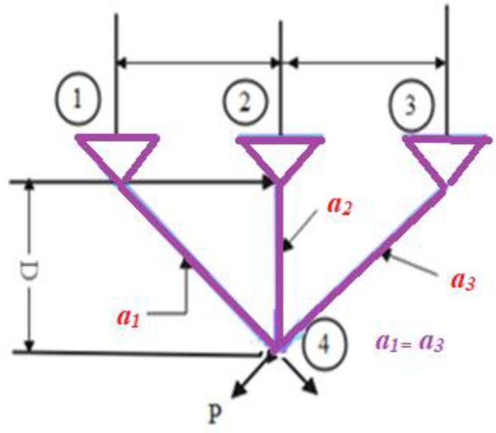
Three-bar truss engineering
Table 20.
Comparison of hSMA-SA results for speed reducer optimization with other techniques
| Competitive techniques | Optimal values for variables | Optimum fitness | ||||||
|---|---|---|---|---|---|---|---|---|
| x1 | x2 | x3 | x4 | x5 | x6 | x7 | ||
| Proposed hSMA-SA | 3.5 | 0.7 | 17 | 7.3 | 7.715380 | 3.350218 | 5.286654 | 2994.474041 |
| HS [98] | 3.520124 | 0.7 | 17 | 8.37 | 7.8 | 3.366970 | 5.288719 | 3029.002 |
| MFO [34] | 3.507524 | 0.7 | 17 | 7.302397 | 7.802364 | 3.323541 | 5.287524 | 3009.571 |
| GSA [20] | 3.600000 | 0.7 | 17 | 8.3 | 7.8 | 3.369658 | 5.289224 | 3051.120 |
| HHO-SCA [54] | 3.506119 | 0.7 | 17 | 7.3 | 7.99141 | 3.452569 | 5.286749 | 3029.873076 |
| GA [165] | 3.510253 | 0.7 | 17 | 8.35 | 7.8 | 3.362201 | 5.287723 | 3067.561 |
| PSO [164] | 3.500019 | 0.7 | 17 | 8.3 | 7.8 | 3.352412 | 5.286715 | 3005.763 |
| OBSCA | 3.0879 | 0.7550 | 26.4738 | 7.3650 | 7.9577 | 3.4950 | 5.2312 | 3056.3122 |
| SCA | 3.508755 | 0.7 | 17 | 7.3 | 7.8 | 3.461020 | 5.289213 | 3030.563 |
where l = 100 cm, P = 2KN/cm2, ρ = 2 KN/cm2
Welded beam
This issue is represented in Fig. 22 [173]. The major goal is to reduce the production costs of the welded beam. (1) Bar height (h) is represented by z4, (2) weld thickness (t) is represented by z3, (3) bar length (L) is represented by z2, and (4) bar thickness (b) is represented by z1; these are the four variables that are subjected to buckling bar (Pc), end beam deflection (d), side restrictions and shear stress (s), and bending beam stress (h). Equations (16) to (18f) show the welded beam optimization design equations. The findings of hSMA-SA are measured with known techniques in Table 21. According to the investigation’s findings, the proposed approach is more capable of managing welded beam design with extreme precision (Table 22).
Fig. 22.
Welded mechanical beam model
Table 21.
Comparison of hSMA-SA results for three-bar truss optimization with known techniques
| Competitive techniques | Optimal values for variables | Optimum weight | |
|---|---|---|---|
| X1 | X2 | ||
| Proposed hSMA-SA | 0.767861026 | 0.470855717 | 264.2694671 |
| Ray and Liew [166] | 0.788621037 | 0.408401334 | 263.8958466 |
| Hernandez | 0.788 | 0.408 | 263.9 |
| CS [167] | 0.789 | 0.409 | 263.972 |
| Ray and Saini [168] | 0.795 | 0.398 | 264.3 |
| HHO-SCA [54] | 0.788498 | 0.40875 | 263.8958665 |
| Gandomi [169] | 0.78867 | 0.40902 | 263.9716 |
| CSA [170] | 0.788638976 | 0.408350573 | 263.895844337 |
| GWO-SA [171] | 0.789 | 0.408 | 263.896 |
| MBA [169] | 0.789 | 0.409 | 263.896 |
| WDE [52] | 0.515535107819326 | 0.0156341500434795 | 2.639297829829848E+02 |
| ALO [152] | 0.789 | 0.408 | 263.8958434 |
| DEDS [172] | 0.789 | 0.408 | 263.896 |
| Raj et al. | 0.789764410 | 0.405176050 | 263.89671 |
Table 22.
Comparison of hSMA-SA results for welded beam optimization design with known techniques
| Competitive techniques | Optimal values for variables | Optimum cost | |||
|---|---|---|---|---|---|
| h | l | t | b | ||
| Proposed hSMA-SA | 0.205727302 | 3.471126735 | 9.035476564 | 0.205781951 | 1.725134404 |
| HS [98] | 0.2442 | 6.2231 | 8.2915 | 0.2443 | 2.3807 |
| PSO [164] | 0.197411 | 3.315061 | 10.00000 | 0.201395 | 1.820395 |
| Approx | 0.2444 | 6.2189 | 8.2189 | 0.2444 | 2.3815 |
| CDE [157] | 0.203137 | 3.542998 | 9.033498 | 0.206179 | 1.733462 |
| David | 0.2434 | 6.2552 | 8.2915 | 0.2444 | 2.3841 |
| GSA [20] | 0.1821 | 3.857 | 10 | 0.2024 | 1.88 |
| (PSOStr) [174] | 0.2015 | 3.526 | 9.041398 | 0.205706 | 1.731186 |
| HHO-SCA [54] | 0.190086 | 3.696496 | 9.386343 | 0.204157 | 1.779032249 |
| MFO [34] | 0.203567 | 3.443025 | 9.230278 | 0.212359 | 1.732541 |
| Gandomi et al. (FA) [175] | 0.2015 | 3.562 | 9.0414 | 0.2057 | 1.73121 |
| SCA | 0.204695 | 3.536291 | 9.004290 | 0.210025 | 1.759173 |
Let us consider
| 16 |
| 17 |
By addressing,
| 17a |
| 17b |
| 17c |
| 17d |
| 17e |
| 17f |
| 17g |
Range of variables:
Here,
| 18a |
| 18b |
| 18c |
| 18d |
| 18e |
| 18f |
Gear train design
This is one of the various engineering difficulties that comprise four variables and a tooth ratio, as spotted in Fig. 23 [153]. The architectural design’s general purpose is to help reduce the scalar value of the gears and the teeth ratio as much as feasible. As an outcome, each gear’s teeth are handled as design variables throughout the process. Table 23 shows the analytical results for a comparison of hSMA-SA with other methodologies. The suggested method is more successful in determining the gear train ratio, according to the observations. The following is a model for the required formulas:
Fig. 23.

Gear train optimization design
Table 23.
Comparison of hSMA-SA results for gear train optimization design with known techniques
| Competitive techniques | Optimal values for variables | Gear ratio | Optimum fitness | |||
|---|---|---|---|---|---|---|
| x1 (Td) | x2 (Tb) | x3 (Ta) | x4 (Tf) | |||
| Proposed hSMA-SA | 17.39759773 | 12.00546725 | 12 | 57.39404929 | NA | 2.70E−11 |
| IMFO [176] | 19 | 14 | 34 | 50 | NA | 3.0498E−13 |
| MARS [177] | 19 | 16 | 43 | 49 | 0.1442 | 2.7E−12 |
| CSA [167] | 19.000 | 16.000 | 43.000 | 49.000 | NA | 2.7008571489E−12 |
| ISA [178] | 19 | 16 | 43 | 49 | NA | 2.701E−12 |
| HGA [179] | 15 | 21 | 59 | 37 | NA | 3.07E−10 |
| MIBBSQP [180] | 18 | 22 | 45 | 60 | 0.146666 | 5.7E−06 |
| MP [181] | 18 | 22 | 45 | 60 | 0.1467 | 5.712E−06 |
| Ahga1 [179] | 13 | 24 | 47 | 46 | NA | 9.92E−10 |
| IDCNLP [182] | 14 | 29 | 47 | 59 | 0.146411 | 4.5E−06 |
| MBA [169] | 16 | 19 | 49 | 43 | 0.1442 | 2.7005E−0.12 |
| MINSLIP [180] | 19 | 16 | 42 | 50 | NA | 2.33E−07 |
| Ahga2 [179] | 13 | 20 | 53 | 34 | NA | 2.31E−11 |
| ALO [152] | 19.00 | 16.00 | 43.00 | 49.00 | NA | 2.7009E−012 |
| CAPSO [169] | 16 | 19 | 49 | 43 | 0.1442 | 2.701E−12 |
Let us consider
| 19 |
To minimize,
| 19a |
Subjected to
| 19b |
Belleville spring
Figure 24 depicts this problem. This is a method for reducing the issue by picking a parameter that already survives in the defined variable ratio limits. The major goal of this task is to reduce the weight while staying within the limitations. Deflection, deflection height, the interior and exterior portions of the diameter, compressive forms of stresses, and slope will all be altered when the limitations are applied. The spring height (SpH), exterior part diameter (DimE), internal part diameter (DimI), and Belleville spring thickness (SpT) of a Belleville spring are all built with minimal weight. The comparative findings are shown in Table 24. The recommended technique is more successful in solving the spring design challenge, according to observations. The formulae are listed as
| 20 |
Fig. 24.
Belleville spring engineering design
Table 24.
Comparison of hSMA-SA results for Belleville spring optimization with known techniques
Subjected to
| 21 |
| 21a |
| 21b |
| 21c |
| 21d |
| 21e |
| 21f |
where
PMaX = 5400 lb.
P = 30e6 psi, = 0.2 in, = 0.3, G = 200 Kpsi, H = 2 in, DimMAX = 12.01 in, ,
Cantilever beam design
The goal of this civil engineering task, as shown in Fig. 25, is to reduce beam weight as much as possible. There are five distinct types of forms in this problem [173]. As seen in Eq. (22), the key objective is to pull down the beam’s weight. The complete design configuration consists of structural features of five elements that must be kept unchanged, with the beam thickness remaining constant, in order to reach the ultimate optimal solution, which is illustrated by Eqs. (33–34). The findings are compared to those obtained using various approaches in Table 25. hSMA-SA outperformed other approaches in terms of beam weight reduction. The mathematics are shown as follows:
| 22 |
Fig. 25.
Design of cantilever beam
Table 25.
Comparison of hSMA-SA outcomes for cantilever beam optimization with known techniques
| Competitive techniques | Optimal values for variables | Optimum weight | ||||
|---|---|---|---|---|---|---|
| L1 | L2 | L3 | L4 | L5 | ||
| Proposed hSMA-SA | 5.982032535 | 4.846178775 | 4.491073327 | 3.48171237 | 2.138830846 | 1.303294886 |
| HHO-PS [50] | 5.978829 | 4.876628 | 4.464572 | 3.479744 | 2.139358 | 1.303251 |
| IMFO [176] | 5.97822 | 4.87623 | 4.46610 | 3.47945 | 2.13912 | 1.30660 |
| SMA [3] | 6.017757 | 5.310892 | 4.493758 | 3.501106 | 2.150159 | 1.339957 |
| GCA_I [24] | 6.0100 | 5.3000 | 4.4900 | 3.4900 | 2.1500 | 1.3400 |
| GWO-SA [171] | 5.9854 | 4.87 | 4.4493 | 3.5172 | 2.1187 | 1.3033 |
| MMA [183] | 6.0100 | 5.3000 | 4.4900 | 3.4900 | 2.1500 | 1.3400 |
| MVO [24] | 6.02394022154 | 5.30301123355 | 4.4950113234 | 3.4960223242 | 2.15272617 | 1.3399595 |
| CS [184] | 6.0089 | 5.3049 | 4.5023 | 3.5077 | 2.1504 | 1.33999 |
| SOS [185] | 6.01878 | 5.30344 | 4.49587 | 3.49896 | 2.15564 | 1.33996 |
| HHO-SCA [54] | 5.937725 | 4.85041 | 4.622404 | 3.45347 | 2.089114 | 1.30412236 |
By addressing,
| 23 |
Ranges of variables are .
Rolling element bearing
The target is to augment the bearing capability of the rolling element, as indicated in Fig. 26 [186]. The engineering design issue comprises a total of 10 decision variables that are used to determine the best bearing design for increasing load-carrying capacity. (1) Diameter of pitch (DimP), (2) diameter of Ball (DimB), (3) ball numbers (NB), (4) curvature coefficient of the outer raceway, and (5) curvature coefficient of inner raceway are the five variables that are given substantial importance, while the remaining five variables (KDMin, KDMax, ε, e, and f) are only assessed for discrete integers and influence interior section of the geometry circuitously. The findings of hSMA-SA are compared with various approaches for this problem in Table 26. Equations (24a through 25c) show the mathematical equations for this design challenge.
Fig. 26.
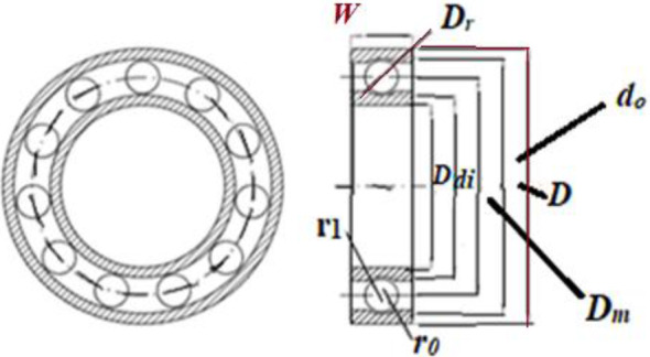
Design of rolling bearing
Table 26.
Comparison of hSMA-SA results for rolling element beam optimization with known techniques
| Competitive algorithms | Optimal values for variables | Optimum fitness | |||||||||
|---|---|---|---|---|---|---|---|---|---|---|---|
| r1 | r2 | r3 | r4 | r5 | r6 | r7 | r8 | r9 | r10 | ||
| Proposed hSMA-SA | 125.7224792 | 21.42329479 | 11.00114251 | 0.515 | 0.515000037 | 0.471814754 | 0.615593477 | 0.300001854 | 0.098010023 | 0.607557895 | − 85,539.05618 |
| SHO [46] | 125 | 21.40732 | 10.93268 | 0.515 | 0.515 | 0.4 | 0.7 | 0.3 | 0.2 | 0.6 | 85,054.532 |
| HHO [78] | 125.00 | 21.00 | 11.092073 | 0.51500 | 0.51500 | 0.4000 | 0.6000 | 0.3000 | 0.050474 | 0.600 | 83,011.88329 |
| WCA [187] | 125.721167 | 21.42300 | 1.001030 | 0.515000 | 0.515000 | 0.401514 | 0.659047 | 0.300032 | 0.040045 | 0.600000 | 85,538.48 |
| PVS [188] | 125.719060 | 21.425590 | 11.000000 | 0.515000 | 0.515000 | 0.400430 | 0.680160 | 0.300000 | 0.079990 | 0.700000 | 81,859.741210 |
| SCA [167] | 125 | 21.03287 | 10.96571 | 0.515 | 0.515 | 0.5 | 0.7 | 0.3 | 0.027780 | 0.62912 | 83,431.117 |
| MFO [34] | 125 | 21.03287 | 10.96571 | 0.515 | 0.515000 | 0.5 | 0.67584 | 0.300214 | 0.02397 | 0.61001 | 84,002.524 |
| MVO [24] | 125.6002 | 21.32250 | 10.97338 | 0.515 | 0.515000 | 0.5 | 0.68782 | 0.301948 | 0.03617 | 0.61061 | 84,491.266 |
For maximizing,
| 24a |
If
| 24b |
If .
Addressing,
| 25 |
| 25a |
| 25b |
| 25c |
| 25d |
| 25e |
| 25f |
| 25g |
| 25h |
| 25i |
Here,
and
I beam design
Essentially, the problem tries to reduce the vertical I beam deviation by changing the four parameters of the vertical I beam. Figure 27 depicts the four parameters br, he, twi, and tfo. According to [189], in array to achieve the proportions of the beam indicated in the picture, geometric and strength constraints must be satisfied in order to optimize using the following criteria: (1) when a beam is displaced by applying force, its cross-section lowers its volume for a given length. (2) When the beam is moved by applying force, there is a static deflection to be recorded. In Eqs. (26–28), the mathematical formulas are given. The investigative outcomes of hSMA-SA are measured with other well-known procedures in Table 27.
Fig. 27.
I beam structure
Table 27.
Comparison of hSMA-SA results for I beam optimization with known techniques
| Competitive techniques | Optimal values for variables | Optimum fitness | |||
|---|---|---|---|---|---|
| (br) × 1 | (he) × 2 | (twi) × 3 | (tfo) × 4 | ||
| Proposed hSMA-SA | 50 | 80 | 1.764705807 | 5 | 0.006625958 |
| BWOA [190] | 50.00 | 80.00 | 1.76470588 | 5.00 | 0.00625958 |
| SMA [3] | 49.998845 | 79.994327 | 1.764747 | 4.999742 | 0.006627 |
| HHO-PS [50] | 50.00 | 80.00 | 1.764706 | 5.00 | 0.006626 |
| CS [184] | 50.0000 | 80.0000 | 0.9000 | 2.3217 | 0.0131 |
| MFO [34] | 50.000 | 80.000 | 1.7647 | 5.000 | 0.0066259 |
| SOS [185] | 50.0000 | 80.0000 | 0.9000 | 2.3218 | 0.0131 |
| CSA [167] | 49.99999 | 80 | 0.9 | 2.3217923 | 0.013074119 |
| ARMS [191] | 37.05 | 80 | 1.71 | 2.31 | 0.131 |
| Improved ARMS [191] | 48.42 | 79.99 | 0.9 | 2.4 | 0.131 |
Consider
| 26 |
| 27 |
| 28 |
Variable range
Tension/compression spring design problem
This issue is indicated in Fig. 28 and is part of the mechanical engineering problem [173]. The key feature of the plan is that it minimizes the spring weight. Three sorts of variable designs are required to address this problem: diameter of wire (dwi), diameter of mean coil (Cdia), and active coil number (ACN). The size of the surge, the minimum variation, and the shear stress constraints will all have a part in the design. The numerical for this problem are shown in Eqs. (29)–(30d). When the findings of hSMA-SA are compared to those of other approaches, as shown in Table 28, it is clear that hSMA-SA effectively decreases the spring’s weight by a little amount.
Fig. 28.
Spring engineering tension/compression design
Table 28.
Comparison of hSMA-SA results for the spring engineering tension/compression with known techniques
| Competitive techniques | Optimal values for variables | Optimum weight | ||
|---|---|---|---|---|
| dwi | Cdia | ACN | ||
| Proposed hSMA-SA | 0.050058749 | 0.3187474 | 13.91919024 | 0.012715329 |
| GA [165] | 0.05010 | 0.310111 | 14.0000 | 0.013036251 |
| PSO [164] | 0.05000 | 0.3140414 | 15.0000 | 0.013192580 |
| DELC [159] | 0.051689061 | 0.356717741 | 11.28896566 | 0.012665233 |
| IMFO [176] | 0.051688973 | 0.356715627 | 11.289089342 | 0.012665233 |
| AIS-GA | 0.0516608 | 0.3560323 | 11.329555 | 0.0126666 |
| HS [98] | 0.05025 | 0.316351 | 15.23960 | 0.012776352 |
| HHO-SCA [54] | 0.054693 | 0.433378 | 7.891402 | 0.012822904 |
| CDE [157] | 0.051609 | 0.354714 | 11.410831 | 0.0126702 |
| G-QPSO [155] | 0.051515 | 0.352529 | 11.538862 | 0.012665 |
| GSA [20] | 0.05000 | 0.317312 | 14.22867 | 0.012873881 |
| BCMO [154] | 0.0516597413 | 0.3560124935 | 11.3304429494 | 0.012665 |
| SCA [167] | 0.050780 | 0.334779 | 12.72269 | 0.012709667 |
| MALO [192] | 0.051759 | 0.358411 | 11.191500 | 0.0126660 |
| MVO [24] | 0.05000 | 0.315956 | 14.22623 | 0.012816930 |
| HHO-PS [50] | 0.051682 | 0.356552 | 11.29867 | 0.012665 |
| MFO [34] | 0.05000 | 0.313501 | 14.03279 | 0.012753902 |
| VCS [193] | 0.051685684299756 | 0.356636508703361 | 11.29372966824506 | 0.012665222962643 |
| BRGA | 0.05167471 | 0.35637260 | 11.3092294 | 0.012665237 |
| WCA [187] | 0.051680 | 0.356522 | 11.300410 | 0.012665 |
| MBA [169] | 0.051656 | 0.355940 | 11.344665 | 0.012665 |
| HEAA | 0.0516895376 | 0.3567292035 | 11.288293703 | 0.012665233 |
Let us consider
| 29 |
But to minimize,
| 30 |
| 30a |
| 30b |
| 30c |
| 30d |
Ranges of variables are .
Multi-disk clutch brake (discrete variables)
The crucial technological challenge is presented in Fig. 29 is the multi-disk clutch brake design difficulty [194]. The target is to minimize or maximize weight; anyways it involves five discrete variables: friction surface number (Fsn), disc thickness (DTh), radius of outer surface (Osr), actuating force form (Fac), and radius of inner surface (Isr). Equations (31) to (34) describe the equations for this problem. Table 29 measures the outcomes of hSMA-SA with other methods, demonstrating that hSMA-SA feat known approaches in view of reaching optimal fitness. The design is provided with mathematical equations as follows:
Fig. 29.

Multiple clutch brake design
Table 29.
Comparison of hSMA-SA results for multidisc clutch optimization design with known techniques
| Competitive techniques | Optimal values for variables | Optimum fitness | ||||
|---|---|---|---|---|---|---|
| × 1 | × 2 | × 3 | × 4 | × 5 | ||
| Proposed hSMA-SA | 69.99997189 | 90 | 1.5 | 999.9999999 | 2.312785172 | 0.389654341 |
| HHO [78] | 69.999999 | 90.00 | 1.00 | 1000.00 | 2.312781994 | 0.259768993 |
| TLBO [50] | 70 | 90 | 3 | 810 | 1 | 0.3136566 |
| WCA [187] | 70.00 | 90.00 | 1.00 | 910.000 | 3.00 | 0.313656 |
| HHO-PS [50] | 76.594 | 96.59401 | 1.5 | 1000 | 2.13829 | 0.389653 |
| MBFPA [195] | 70 | 90 | 1 | 600 | 2 | 0.235242457900804 |
| PVS [188] | 70 | 90 | 1 | 980 | 3 | 0.31366 |
| HHO-SCA [54] | 70 | 90 | 2.312785 | 1000 | 1.5 | 0.389653842 |
| NSGA-II | 70 | 90 | 3 | 1000 | 1.5 | 0.4704 |
| MADE [54] | 70.00 | 90 | 3 | 810 | 1 | 0.3136566 |
The mathematics is provided:
| 31 |
where
Subjected to
| 32 |
| 32a |
| 32b |
| 32c |
| 32d |
| 32e |
| 32f |
Here,
Conclusion
In this work of research, a combination of two optimizers has been fruitfully launched a hybridized optimizer named slime mould-simulated annealing algorithm, which relies on the character of slime mould and enacts the uniqueness of the phase of oscillation (Fig. 30). In the global search region, it uses adaptive weights for wave propagation to identify the best solution. The newly created approach has been examined for a variety of 11 interdisciplinary design problems and traditional benchmark optimization challenges, involving 6—unimodal, 5—multimodal, and 5—fixed-dimension benchmark problems. It has been empirically found that the approach is effective to find the solution inside the global search space after testing the competence of the suggested techniques for typical benchmarks and interdisciplinary engineering design issues. It has been advised that the suggested hybrid optimizer be collectively approved to crack tough special engineering design tasks in the global search space depending on practical findings and comparison study with known approaches. Furthermore, these hybrid variations may be used to tackle the actual power system’s multi-area economic load dispatch problem. The proposed algorithm is taking too much time for high dimensions objective function and going out of memory for 140 units economic load dispatch problem. Hence, the computational capacity of the suggested algorithm is slow for higher dimension benchmark problems. The proposed algorithm proved in obtaining influential and optimal solutions. In the outlook, the proposed SMA variant may be appreciably used to find solutions for different types of engineering and design optimization problems also single-area and multi-area economic load dispatch, generation scheduling problem, and auto-generation control issues of practical power systems; it may be utilized to find solutions for power dispatch issues incorporating PEVs, BEVs, and renewable energy sources.
Declarations
Conflict of interest
All the authors contributed to (a) the study’s idea and design, as well as the data analysis and interpretation; (b) the article’s writing or critical revision for key intellectual content; and (c) the final version’s approval. This work has not been submitted to, and is not currently being reviewed by, any other journal or publication venue. The writers are not affiliated with any entity that has a direct or indirect financial interest in the manuscript’s subject matter. There are no writers who have declared a conflict of interest.
Footnotes
Publisher's Note
Springer Nature remains neutral with regard to jurisdictional claims in published maps and institutional affiliations.
Contributor Information
Leela Kumari Ch, Email: leela.41800411@lpu.in.
S. K. Bath, Email: sjkbath.gzsccet@mrsptu.ac.in
References
- 1.Chen H, Jiao S, Heidari AA, Wang M, Chen X, Zhao X. An opposition-based sine cosine approach with local search for parameter estimation of photovoltaic models. Energy Convers Manag. 2019;195(May):927–942. doi: 10.1016/j.enconman.2019.05.057. [DOI] [Google Scholar]
- 2.Osher SJ et al (2018) Laplacian smooth gradient descent. pp 1–28. 10.48550/ARXIV.1806.06317
- 3.Li S, Chen H, Wang M, Heidari AA, Mirjalili S. Slime mould algorithm: a new method for stochastic optimization. Future Gener Comput Syst. 2020;111:300–323. doi: 10.1016/j.future.2020.03.055. [DOI] [Google Scholar]
- 4.Sun K, Jia H, Li Y, Jiang Z. Hybrid improved slime mould algorithm with adaptive β hill climbing for numerical optimization. J Intell Fuzzy Syst. 2021;40(1):1667–1679. doi: 10.3233/JIFS-201755. [DOI] [Google Scholar]
- 5.Gao ZM, Zhao J, Yang Y, Tian XJ. The hybrid grey wolf optimization-slime mould algorithm. J Phys Conf Ser. 2020 doi: 10.1088/1742-6596/1617/1/012034. [DOI] [Google Scholar]
- 6.Zhao J, Gao ZM, Sun W. The improved slime mould algorithm with Levy flight. J Phys Conf Ser. 2020 doi: 10.1088/1742-6596/1617/1/012033. [DOI] [Google Scholar]
- 7.Zhao J, Gao ZM. The chaotic slime mould algorithm with Chebyshev map. J Phys Conf Ser. 2020 doi: 10.1088/1742-6596/1631/1/012071. [DOI] [Google Scholar]
- 8.Cui Z, Hou X, Zhou H, Lian W, Wu J (2020) Modified slime mould algorithm via Levy flight, November, pp 1109–1113. 10.1109/cisp-bmei51763.2020.9263669.
- 9.Izci D, Ekinci S, Zeynelgil HL, Hedley J. Performance evaluation of a novel improved slime mould algorithm for direct current motor and automatic voltage regulator systems. Trans Inst Meas Control. 2021;44(2):435–456. doi: 10.1177/01423312211037967. [DOI] [Google Scholar]
- 10.Zhao J, Gao ZM. The hybridized Harris hawk optimization and slime mould algorithm. J Phys Conf Ser. 2020 doi: 10.1088/1742-6596/1682/1/012029. [DOI] [Google Scholar]
- 11.Gao ZM, Zhao J, Li SR. The improved slime mould algorithm with cosine controlling parameters. J Phys Conf Ser. 2020 doi: 10.1088/1742-6596/1631/1/012083. [DOI] [Google Scholar]
- 12.Monismith DR, Mayfield BE (2008) Slime mould as a model for numerical optimization. 2008 IEEE Swarm Intell. Symp. SIS 2008, no. January. 10.1109/SIS.2008.4668295
- 13.Premkumar M, Jangir P, Sowmya R, Alhelou HH, Heidari AA, Chen H. MOSMA: multi-objective slime mould algorithm based on elitist non-dominated sorting. IEEE Access. 2021;9:3229–3248. doi: 10.1109/ACCESS.2020.3047936. [DOI] [Google Scholar]
- 14.Li K, Torres CE, Thomas K, Rossi LF, Shen CC. Slime mould inspired routing protocols for wireless sensor networks. Swarm Intell. 2011;5(3–4):183–223. doi: 10.1007/s11721-011-0063-y. [DOI] [Google Scholar]
- 15.Qian T, Zhang Z, Gao C, Wu Y, Liu Y (2013) An ant colony system based on the physarum network. Lect. Notes Comput. Sci. (including Subser. Lect. Notes Artif. Intell. Lect. Notes Bioinformatics), vol 7928 LNCS, no PART 1, pp 297–305. 10.1007/978-3-642-38703-6_35
- 16.Schmickl T, Crailsheim K (2007) A navigation algorithm for swarm robotics inspired by slime mould aggregation. Lect. Notes Comput. Sci. (including Subser. Lect. Notes Artif. Intell. Lect. Notes Bioinformatics), vol 4433 LNCS, no September, pp 1–13. 10.1007/978-3-540-71541-2_1
- 17.Becker M (2016) On the efficiency of nature-inspired algorithms for generation of fault-tolerant graphs. In: Proceedings of 2015 IEEE international conference system man, cybernetics. SMC 2015, no. September, pp 1657–1663. 10.1109/SMC.2015.292
- 18.Brabazon A, McGarraghy S. Slime mould foraging: an inspiration for algorithmic design. Int J Innov Comput Appl. 2020;11(1):30–45. doi: 10.1504/IJICA.2020.105316. [DOI] [Google Scholar]
- 19.Suid MH, Ahmad MA, Ismail MRTR, Ghazali MR, Irawan A, Tumari MZ (2019) An improved sine cosine algorithm for solving optimization problems. In: Proceedings of 2018 IEEE conference system process control. ICSPC 2018, pp 209–213. 10.1109/SPC.2018.8703982
- 20.Rashedi E, Nezamabadi-pour H, Saryazdi S. GSA: a gravitational search algorithm. Inf Sci (Ny) 2009;179(13):2232–2248. doi: 10.1016/j.ins.2009.03.004. [DOI] [Google Scholar]
- 21.Formato RA. Central force optimization: a new metaheuristic with applications in applied electromagnetics. Prog Electromagn Res. 2007;77:425–491. doi: 10.2528/PIER07082403. [DOI] [Google Scholar]
- 22.Mosavi MR, Khishe M, Naseri MJ, Parvizi GR, Ayat M. Multi-layer perceptron neural network utilizing adaptive best-mass gravitational search algorithm to classify sonar dataset. Arch Acoust. 2019;44(1):137–151. doi: 10.24425/aoa.2019.126360. [DOI] [Google Scholar]
- 23.Kaveh A, Talatahari S. A novel heuristic optimization method: charged system search. Acta Mech. 2010;213(3–4):267–289. doi: 10.1007/s00707-009-0270-4. [DOI] [Google Scholar]
- 24.Mirjalili S, Mirjalili SM, Hatamlou A. Multi-verse optimizer: a nature-inspired algorithm for global optimization. Neural Comput Appl. 2016;27(2):495–513. doi: 10.1007/s00521-015-1870-7. [DOI] [Google Scholar]
- 25.Koza JR, Rice JP. Automatic programming of robots using genetic programming. Proc Tenth Natl Conf Artif Intell. 1992;92:194–207. [Google Scholar]
- 26.Yao X, Liu Y, Lin G. Evolutionary programming made faster. IEEE Trans Evol Comput. 1999;3(2):82–102. doi: 10.1109/4235.771163. [DOI] [Google Scholar]
- 27.Simon D. Biogeography-based optimization. IEEE Trans Evol Comput. 2008;12(6):702–713. doi: 10.1109/TEVC.2008.919004. [DOI] [Google Scholar]
- 28.Fleetwood K (2004) An introduction to differential evolution. In: Proceedings of mathematics and statistics of complex systems (MASCOS) one day symposium, 26th November, Brisbane, Australia. pp 785–791
- 29.Mirjalili S. Genetic algorithm. Stud Comput Intell. 2019;780:43–55. doi: 10.1007/978-3-319-93025-1_4. [DOI] [Google Scholar]
- 30.He X, Zheng Z, Zhou Y. MMES: mixture model based evolution strategy for large-scale optimization. IEEE Trans Evol Comput. 2020 doi: 10.1109/tevc.2020.3034769. [DOI] [Google Scholar]
- 31.Qiao W, Moayedi H, Foong LK. Nature-inspired hybrid techniques of IWO, DA, ES, GA, and ICA, validated through a k-fold validation process predicting monthly natural gas consumption. Energy Build. 2020 doi: 10.1016/j.enbuild.2020.110023. [DOI] [Google Scholar]
- 32.Beni G, Wang J. Swarm intelligence in cellular robotic systems. Robot Biol Syst Towar New Bionics. 1993 doi: 10.1007/978-3-642-58069-7_38. [DOI] [Google Scholar]
- 33.Mafarja MM, Mirjalili S. Hybrid binary ant lion optimizer with rough set and approximate entropy reducts for feature selection. Soft Comput. 2019;23(15):6249–6265. doi: 10.1007/s00500-018-3282-y. [DOI] [Google Scholar]
- 34.Mirjalili S. Moth-flame optimization algorithm: a novel nature-inspired heuristic paradigm. Knowl Based Syst. 2015;89:228–249. doi: 10.1016/j.knosys.2015.07.006. [DOI] [Google Scholar]
- 35.Karaboga D, Basturk B. A powerful and efficient algorithm for numerical function optimization: artificial bee colony (ABC) algorithm. J Glob Optim. 2007;39(3):459–471. doi: 10.1007/s10898-007-9149-x. [DOI] [Google Scholar]
- 36.Heidari AA, Mirjalili S, Faris H, Aljarah I, Mafarja M, Chen H. Harris hawks optimization: algorithm and applications. Future Gener Comput Syst. 2019;97:849–872. doi: 10.1016/j.future.2019.02.028. [DOI] [Google Scholar]
- 37.Pan WT. A new fruit fly optimization algorithm: taking the financial distress model as an example. Knowl Based Syst. 2012;26:69–74. doi: 10.1016/j.knosys.2011.07.001. [DOI] [Google Scholar]
- 38.Dorigo M, Blum C. Ant colony optimization theory: a survey. Theor Comput Sci. 2005;344(2–3):243–278. doi: 10.1016/j.tcs.2005.05.020. [DOI] [Google Scholar]
- 39.Mirjalili S, Mirjalili SM, Lewis A. Grey wolf optimizer. Adv Eng Softw. 2014 doi: 10.1016/j.advengsoft.2013.12.007. [DOI] [Google Scholar]
- 40.Rao RV, Savsani VJ, Vakharia DP. Teaching-learning-based optimization: an optimization method for continuous non-linear large scale problems. Inf Sci (Ny) 2012;183(1):1–15. doi: 10.1016/j.ins.2011.08.006. [DOI] [Google Scholar]
- 41.Glover F, Taillard E. A user's guide to tabu search. Ann Oper Res. 1993;41(1):1–28. doi: 10.1007/BF02078647. [DOI] [Google Scholar]
- 42.Lin L, Gen M. Auto-tuning strategy for evolutionary algorithms: Balancing between exploration and exploitation. Soft Comput. 2009;13(2):157–168. doi: 10.1007/s00500-008-0303-2. [DOI] [Google Scholar]
- 43.Whitley D, Rowe J (2008) Focused no free lunch theorems. GECCO’08 Proceedings of 10th annual conference genetics evolution computing. pp 811–818. 10.1145/1389095.1389254
- 44.Wolpert DH, Macready WG. No free lunch theorems for optimization. IEEE Trans Evol Comput. 1997;1(1):67–82. doi: 10.1109/4235.585893. [DOI] [Google Scholar]
- 45.Huang KW, Wu ZX. CPO: a crow particle optimization algorithm. Int J Comput Intell Syst. 2018;12(1):426–435. doi: 10.2991/ijcis.2018.125905658. [DOI] [Google Scholar]
- 46.Dhiman G, Kumar V. Spotted hyena optimizer: a novel bio-inspired based metaheuristic technique for engineering applications. Adv Eng Softw. 2017;114:48–70. doi: 10.1016/j.advengsoft.2017.05.014. [DOI] [Google Scholar]
- 47.Kalananda VKRA, Komanapalli VLN. A combinatorial social group whale optimization algorithm for numerical and engineering optimization problems. Appl Soft Comput. 2021;99:106903. doi: 10.1016/j.asoc.2020.106903. [DOI] [Google Scholar]
- 48.Dhiman G, Kumar V. Multi-objective spotted hyena optimizer: a multi-objective optimization algorithm for engineering problems. Knowl Based Syst. 2018;150(March):175–197. doi: 10.1016/j.knosys.2018.03.011. [DOI] [Google Scholar]
- 49.Hu K, Jiang H, Ji CG, Pan Z. A modified butterfly optimization algorithm: an adaptive algorithm for global optimization and the support vector machine. Expert Syst. 2020 doi: 10.1111/exsy.12642. [DOI] [Google Scholar]
- 50.Krishna AB, Saxena S, Kamboj VK. A novel statistical approach to numerical and multidisciplinary design optimization problems using pattern search inspired Harris hawks optimizer. Neural Comput Appl. 2021;33(12):7031–7072. doi: 10.1007/s00521-020-05475-5. [DOI] [Google Scholar]
- 51.Kumar V, Kaur A. Binary spotted hyena optimizer and its application to feature selection. J Ambient Intell Humaniz Comput. 2020;11(7):2625–2645. doi: 10.1007/s12652-019-01324-z. [DOI] [Google Scholar]
- 52.Zamani H, Nadimi-shahraki MH. Enhancement of Bernstain-search differential evolution algorithm to solve constrained engineering problems. Int J Comput Sci Eng (IJCSE) 2020;9(6):386–396. [Google Scholar]
- 53.Meng Z, Li G, Wang X, Sait SM, Yıldız AR. A comparative study of metaheuristic algorithms for reliability-based design optimization problems. Arch Comput Methods Eng. 2020 doi: 10.1007/s11831-020-09443-z. [DOI] [Google Scholar]
- 54.Kamboj VK, Nandi A, Bhadoria A, Sehgal S. An intensify Harris Hawks optimizer for numerical and engineering optimization problems. Appl Soft Comput J. 2020;89:106018. doi: 10.1016/j.asoc.2019.106018. [DOI] [Google Scholar]
- 55.Che Y, He D. An enhanced seagull optimization algorithm for solving engineering optimization problems. Appl Intell. 2022 doi: 10.1007/s10489-021-03155-y. [DOI] [Google Scholar]
- 56.Li Z, Zhang Q, He Y. Modified group theory-based optimization algorithms for numerical optimization. Appl Intell. 2022 doi: 10.1007/s10489-021-02982-3. [DOI] [Google Scholar]
- 57.Srivastava A, Das DK. Criminal search optimization algorithm: a population-based meta-heuristic optimization technique to solve real-world optimization problems. Arab J Sci Eng. 2022 doi: 10.1007/s13369-021-06446-1. [DOI] [Google Scholar]
- 58.Talatahari B, Azizi M, Talatahari S, Tolouei M, Sareh P. Crystal structure optimization approach to problem solving in mechanical engineering design. Multidiscip Model Mater Struct. 2022 doi: 10.1108/mmms-10-2021-0174. [DOI] [Google Scholar]
- 59.Abdollahzadeh B, Gharehchopogh FS, Mirjalili S. African vultures optimization algorithm: a new nature-inspired metaheuristic algorithm for global optimization problems. Comput Ind Eng. 2021;158(May):107408. doi: 10.1016/j.cie.2021.107408. [DOI] [Google Scholar]
- 60.Karami H, Anaraki MV, Farzin S, Mirjalili S. Flow direction algorithm (FDA): a novel optimization approach for solving optimization problems. Comput Ind Eng. 2021;156(March):107224. doi: 10.1016/j.cie.2021.107224. [DOI] [Google Scholar]
- 61.Barshandeh S, Haghzadeh M. A new hybrid chaotic atom search optimization based on tree-seed algorithm and Levy flight for solving optimization problems. Eng Comput. 2021;37:3079–3122. doi: 10.1007/s00366-020-00994-0. [DOI] [Google Scholar]
- 62.Abdollahzadeh B, Gharehchopogh FS. A multi-objective optimization algorithm for feature selection problems. Eng Comput. 2021 doi: 10.1007/s00366-021-01369-9. [DOI] [Google Scholar]
- 63.Abualigah L, Diabat A, Mirjalili S, Elaziz MA, Gandomi AH. The arithmetic optimization algorithm. Comput Methods Appl Mech Eng. 2021;376:113609. doi: 10.1016/j.cma.2020.113609. [DOI] [Google Scholar]
- 64.Abualigah L, Yousri D, Elaziz MA, Ewees AA, Al-qaness MAA, Gandomi AH. Aquila optimizer: a novel meta-heuristic optimization algorithm. Comput Ind Eng. 2021;157:107250. doi: 10.1016/j.cie.2021.107250. [DOI] [Google Scholar]
- 65.Abdollahzadeh B, Gharehchopogh FS, Mirjalili S. Artificial gorilla troops optimizer: a new nature-inspired metaheuristic algorithm for global optimization problems. Int J Intell Syst. 2021;36(10):5887–5958. doi: 10.1002/int.22535. [DOI] [Google Scholar]
- 66.Abdel-Basset M, Mohamed R, Chakrabortty RK, Ryan MJ, Mirjalili S. An efficient binary slime mould algorithm integrated with a novel attacking-feeding strategy for feature selection. Comput Ind Eng. 2021;153:107078. doi: 10.1016/j.cie.2020.107078. [DOI] [Google Scholar]
- 67.Marfia S, Vigliotti A (2021) 1D SMA models. In: Shape memory alloy engineering. Elsevier, pp 247–290. 10.1016/B978-0-12-819264-1.00008-X
- 68.Izci D, Ekinci S. Comparative performance analysis of slime mould algorithm for efficient design of proportional–integral–derivative controller. Electrica. 2021;21(1):151–159. doi: 10.5152/electrica.2021.20077. [DOI] [Google Scholar]
- 69.Zitouni F, Harous S, Belkeram A, Hammou LEB (2021) The Archerfish hunting optimizer: a novel metaheuristic algorithm for global optimization. 178(1): 1–41. http://arxiv.org/abs/2102.02134
- 70.Ren H, Li J, Chen H, Li CY. Adaptive levy-assisted salp swarm algorithm: analysis and optimization case studies. Math Comput Simul. 2021;181(March):380–409. doi: 10.1016/j.matcom.2020.09.027. [DOI] [Google Scholar]
- 71.Lin SW, Cheng CY, Pourhejazy P, Ying KC. Multi-temperature simulated annealing for optimizing mixed-blocking permutation flowshop scheduling problems. Expert Syst Appl. 2021;165(August 2020):113837. doi: 10.1016/j.eswa.2020.113837. [DOI] [Google Scholar]
- 72.Salgotra R, Singh U, Singh S, Singh G, Mittal N. Self-adaptive salp swarm algorithm for engineering optimization problems. Appl Math Model. 2021;89(November):188–207. doi: 10.1016/j.apm.2020.08.014. [DOI] [Google Scholar]
- 73.Lee J, Perkins D. A simulated annealing algorithm with a dual perturbation method for clustering. Pattern Recognit. 2020 doi: 10.1016/j.patcog.2020.107713. [DOI] [Google Scholar]
- 74.Liu Y, Li R. PSA: a photon search algorithm. J Inf Process Syst. 2020;16(2):478–493. doi: 10.3745/JIPS.04.0168. [DOI] [Google Scholar]
- 75.Rizk-Allah RM, Hassanien AE. A movable damped wave algorithm for solving global optimization problems. Evol Intell. 2019;12(1):49–72. doi: 10.1007/s12065-018-0187-8. [DOI] [Google Scholar]
- 76.Hashim FA, Houssein EH, Mabrouk MS, Al-atabany W. Henry gas solubility optimization: a novel physics-based algorithm. Future Gener Comput Syst. 2019;101:646–667. doi: 10.1016/j.future.2019.07.015. [DOI] [Google Scholar]
- 77.Harifi S, Khalilian M, Mohammadzadeh J, Ebrahimnejad S. Emperor Penguins Colony: a new metaheuristic algorithm for optimization. Evol Intell. 2019;12(2):211–226. doi: 10.1007/s12065-019-00212-x. [DOI] [Google Scholar]
- 78.Heidari AA, Mirjalili S, Faris H, Aljarah I, Mafarja M, Chen H. “Harris hawks optimization: algorithm and applications Harris hawks optimization. Algorithm Appl. 2019 doi: 10.1016/j.future.2019.02.028. [DOI] [Google Scholar]
- 79.Cheraghalipour A, Hajiaghaei-Keshteli M, Paydar MM. Tree Growth Algorithm (TGA): a novel approach for solving optimization problems. Eng Appl Artif Intell. 2018;72(February):393–414. doi: 10.1016/j.engappai.2018.04.021. [DOI] [Google Scholar]
- 80.Ghanem WAHM, Jantan A. Hybridizing artificial bee colony with monarch butterfly optimization for numerical optimization problems. Neural Comput Appl. 2018;30(1):163–181. doi: 10.1007/s00521-016-2665-1. [DOI] [Google Scholar]
- 81.Wahid F, Ghazali R, Shah H. An improved hybrid firefly algorithm for solving optimization problems. Adv Intell Syst Comput. 2018;700:14–23. doi: 10.1007/978-3-319-72550-5_2. [DOI] [Google Scholar]
- 82.Arora S, Singh S. An improved butterfly optimization algorithm with chaos. J Intell Fuzzy Syst. 2017;32(1):1079–1088. doi: 10.3233/JIFS-16798. [DOI] [Google Scholar]
- 83.Shehab M, Khader AT, Al-Betar MA, Abualigah LM (2017) Hybridizing cuckoo search algorithm with hill climbing for numerical optimization problems. In: ICIT 2017—8th international conference information technology proceedings, no. May. pp 36–43. 10.1109/ICITECH.2017.8079912.
- 84.Singh N, Singh SB. A novel hybrid GWO-SCA approach for optimization problems. Eng Sci Technol Int J. 2017;20(6):1586–1601. doi: 10.1016/j.jestch.2017.11.001. [DOI] [Google Scholar]
- 85.Mirjalili S. SCA: a sine cosine algorithm for solving optimization problems. Knowl Based Syst. 2016 doi: 10.1016/j.knosys.2015.12.022. [DOI] [Google Scholar]
- 86.Yazdani M, Jolai F. Lion Optimization Algorithm (LOA): a nature-inspired metaheuristic algorithm. J Comput Des Eng. 2016;3(1):24–36. doi: 10.1016/j.jcde.2015.06.003. [DOI] [Google Scholar]
- 87.Askarzadeh A. A novel metaheuristic method for solving constrained engineering optimization problems: crow search algorithm. Comput Struct. 2016;169:1–12. doi: 10.1016/j.compstruc.2016.03.001. [DOI] [Google Scholar]
- 88.Salimi H. Stochastic fractal search: a powerful metaheuristic algorithm. Knowl Based Syst. 2015;75:1–18. doi: 10.1016/j.knosys.2014.07.025. [DOI] [Google Scholar]
- 89.Farahmandian M, Hatamlou A. Solving optimization problems using black hole algorithm. J Adv Comput Sci Technol. 2015;4(1):68. doi: 10.14419/jacst.v4i1.4094. [DOI] [Google Scholar]
- 90.Ghaemi M, Feizi-Derakhshi MR. Forest optimization algorithm. Expert Syst Appl. 2014;41(15):6676–6687. doi: 10.1016/j.eswa.2014.05.009. [DOI] [Google Scholar]
- 91.Roy S, Chaudhuri SS. Cuckoo search algorithm using Lèvy flight: a review. Int J Mod Educ Comput Sci. 2013;5(12):10–15. doi: 10.5815/ijmecs.2013.12.02. [DOI] [Google Scholar]
- 92.Yang XS, He X. Firefly algorithm: recent advances and applications. Int J Swarm Intell. 2013;1(1):36. doi: 10.1504/ijsi.2013.055801. [DOI] [Google Scholar]
- 93.Yang XS. Bat algorithm: literature review and applications. Int J Bioinspired Comput. 2013;5(3):141–149. doi: 10.1504/IJBIC.2013.055093. [DOI] [Google Scholar]
- 94.Gheraibia Y, Moussaoui A. Recent trends. Appl Artif Intell. 2013 doi: 10.1007/978-3-642-38577-3. [DOI] [Google Scholar]
- 95.Gandomi AH, Alavi AH. Krill herd: a new bio-inspired optimization algorithm. Commun Nonlinear Sci Numer Simul. 2012;17(12):4831–4845. doi: 10.1016/j.cnsns.2012.05.010. [DOI] [Google Scholar]
- 96.Y X-s (2012) Flower pollination algorithm for global optimization. In: Unconventional computation and natural computation. Springer, p 2409. 10.1007/978-3-642-32894-7_27
- 97.Ghodrati A, Lotfi S. A hybrid CS/GA algorithm for global optimization. Adv Intell Soft Comput. 2012;130(1):397–404. doi: 10.1007/978-81-322-0487-9_38. [DOI] [Google Scholar]
- 98.Geem ZW, Kim JH, Loganathan GV. A new heuristic optimization algorithm: harmony search. SIMULATION. 2001;76(2):60–68. doi: 10.1177/003754970107600201. [DOI] [Google Scholar]
- 99.Storn R, Price K. Differential evolution—a simple and efficient heuristic for global optimization over continuous spaces. J Glob Optim. 1997 doi: 10.1023/A:1008202821328. [DOI] [Google Scholar]
- 100.Glover F. Tabu search—part I. Orsa J Comput. 1989;1(3):190–206. doi: 10.1287/ijoc.1.3.190. [DOI] [Google Scholar]
- 101.Li X, Zhang J, Yin M. Animal migration optimization: an optimization algorithm inspired by animal migration behavior. Neural Comput Appl. 2014;24(7–8):1867–1877. doi: 10.1007/s00521-013-1433-8. [DOI] [Google Scholar]
- 102.Mirjalili S. SCA: a sine cosine algorithm for solving optimization problems. Knowl Based Syst. 2016;96:120–133. doi: 10.1016/j.knosys.2015.12.022. [DOI] [Google Scholar]
- 103.He S, Wu QH, Saunders JR. Group search optimizer: an optimization algorithm inspired by animal searching behavior. IEEE Trans Evol Comput. 2009;13(5):973–990. doi: 10.1109/TEVC.2009.2011992. [DOI] [Google Scholar]
- 104.Gandomi AH. Interior search algorithm (ISA): a novel approach for global optimization. ISA Trans. 2014 doi: 10.1016/j.isatra.2014.03.018. [DOI] [PubMed] [Google Scholar]
- 105.Tabari A, Ahmad A. A new optimization method: electro-search algorithm. Comput Chem Eng. 2017;103:1–11. doi: 10.1016/j.compchemeng.2017.01.046. [DOI] [Google Scholar]
- 106.Kaur S, Awasthi LK, Sangal AL, Dhiman G. Tunicate Swarm Algorithm: a new bio-inspired based metaheuristic paradigm for global optimization. Eng Appl Artif Intell. 2020;90:103541. doi: 10.1016/j.engappai.2020.103541. [DOI] [Google Scholar]
- 107.Xu Z, et al. Orthogonally-designed adapted grasshopper optimization: a comprehensive analysis. Expert Syst Appl. 2020 doi: 10.1016/j.eswa.2020.113282. [DOI] [Google Scholar]
- 108.Ahmadianfar I, Bozorg-Haddad O, Chu X. Gradient-based optimizer: a new metaheuristic optimization algorithm. Inf Sci (Ny) 2020;540:131–159. doi: 10.1016/j.ins.2020.06.037. [DOI] [Google Scholar]
- 109.Qais MH, Hasanien HM, Alghuwainem S. Transient search optimization: a new meta-heuristic optimization algorithm. Appl Intell. 2020;50(11):3926–3941. doi: 10.1007/s10489-020-01727-y. [DOI] [Google Scholar]
- 110.Fouad MM, El-Desouky AI, Al-Hajj R, El-Kenawy ESM. Dynamic group-based cooperative optimization algorithm. IEEE Access. 2020;8:148378–148403. doi: 10.1109/ACCESS.2020.3015892. [DOI] [Google Scholar]
- 111.Abedinpourshotorban H, Mariyam S, Beheshti Z. Electromagnetic field optimization: a physics-inspired metaheuristic optimization algorithm. Swarm Evol Comput. 2015 doi: 10.1016/j.swevo.2015.07.002. [DOI] [Google Scholar]
- 112.Zhao W, Zhang Z, Wang L. Manta ray foraging optimization: an effective bio-inspired optimizer for engineering applications. Eng Appl Artif Intell. 2020;87:103300. doi: 10.1016/j.engappai.2019.103300. [DOI] [Google Scholar]
- 113.Khatri A, Gaba A, Rana KPS, Kumar V. A novel life choice-based optimizer. Soft Comput. 2020;24(12):9121–9141. doi: 10.1007/s00500-019-04443-z. [DOI] [Google Scholar]
- 114.Muhammed DA, Saeed SAM, Rashid TA. Improved fitness-dependent optimizer algorithm. IEEE Access. 2020;8:19074–19088. doi: 10.1109/ACCESS.2020.2968064. [DOI] [Google Scholar]
- 115.Seyyedabbasi A, Kiani F. I-GWO and Ex-GWO: improved algorithms of the Grey Wolf Optimizer to solve global optimization problems. Eng Comput. 2021;37(1):509–532. doi: 10.1007/s00366-019-00837-7. [DOI] [Google Scholar]
- 116.Banerjee N, Mukhopadhyay S (2019) HC-PSOGWO: hybrid crossover oriented PSO and GWO based co-evolution for global optimization. In: Proceedings of 2019 IEEE Reg. 10 Symposium TENSYMP 2019, vol 7, pp 162–167. 10.1109/TENSYMP46218.2019.8971231.
- 117.Chen X, Tianfield H, Li K. Self-adaptive differential artificial bee colony algorithm for global optimization problems. Swarm Evol Comput. 2019;45:70–91. doi: 10.1016/j.swevo.2019.01.003. [DOI] [Google Scholar]
- 118.Tejani GG, Kumar S, Gandomi AH. Multi-objective heat transfer search algorithm for truss optimization. Eng Comput. 2021;37(1):641–662. doi: 10.1007/s00366-019-00846-6. [DOI] [Google Scholar]
- 119.Dhawale D, Kamboj VK, Anand P. An improved chaotic Harris Hawks optimizer for solving numerical and engineering optimization problems. Eng Comput. 2021 doi: 10.1007/s00366-021-01487-4. [DOI] [Google Scholar]
- 120.Chauhan S, Vashishtha G, Kumar A. A symbiosis of arithmetic optimizer with slime mould algorithm for improving global optimization and conventional design problem. J Supercomput. 2021 doi: 10.1007/s11227-021-04105-8. [DOI] [Google Scholar]
- 121.Abualigah L, Diabat A, Elaziz MA. Improved slime mould algorithm by opposition-based learning and Levy flight distribution for global optimization and advances in real-world engineering problems. J Ambient Intell Humaniz Comput. 2021 doi: 10.1007/s12652-021-03372-w. [DOI] [Google Scholar]
- 122.Wang S, et al. A hybrid SSA and SMA with mutation opposition-based learning for constrained engineering problems. Comput Intell Neurosci. 2021 doi: 10.1155/2021/6379469. [DOI] [PMC free article] [PubMed] [Google Scholar]
- 123.M. K. Naik, R. Panda, and A. Abraham, “Normalized square difference based multilevel thresholding technique for multispectral images using leader slime mould algorithm,” J. King Saud Univ. - Comput. Inf. Sci., no. xxxx, 2020, doi: 10.1016/j.jksuci.2020.10.030.
- 124.Salama M, Srinivas S. Adaptive neighborhood simulated annealing for sustainability-oriented single machine scheduling with deterioration effect. Appl Soft Comput. 2021;110:107632. doi: 10.1016/j.asoc.2021.107632. [DOI] [Google Scholar]
- 125.Bandyopadhyay R, Basu A, Cuevas E, Sarkar R. Harris Hawks optimisation with simulated annealing as a deep feature selection method for screening of COVID-19 CT-scans. Appl Soft Comput. 2021;111:107698. doi: 10.1016/j.asoc.2021.107698. [DOI] [PMC free article] [PubMed] [Google Scholar]
- 126.Ilhan İ. An improved simulated annealing algorithm with crossover operator for capacitated vehicle routing problem. Swarm Evol Comput. 2021;64:100911. doi: 10.1016/j.swevo.2021.100911. [DOI] [Google Scholar]
- 127.Lalaoui M, El Afia A, Chiheb R. Dynamic simulated annealing with adaptive neighborhood using Hidden Markov Model. In: Yalaoui F, Amodeo L, Talbi E-G, editors. Heuristics for optimization and learning. Cham: Springer International Publishing; 2021. pp. 167–182. [Google Scholar]
- 128.Izci D, Ekinci S, Hekimoğlu B. Fractional-order PID controller design for buck converter system via hybrid Lèvy flight distribution and simulated annealing algorithm. Arab J Sci Eng. 2022 doi: 10.1007/s13369-021-06383-z. [DOI] [Google Scholar]
- 129.Izci D. A novel improved atom search optimization algorithm for designing power system stabilizer. Evol Intell. 2021 doi: 10.1007/s12065-021-00615-9. [DOI] [Google Scholar]
- 130.Eker E, Kayri M, Ekinci S, Izci D. A new fusion of ASO with SA algorithm and its applications to MLP training and DC motor speed control. Arab J Sci Eng. 2021;46(4):3889–3911. doi: 10.1007/s13369-020-05228-5. [DOI] [Google Scholar]
- 131.Howard FL. The life history of Physarum Polycephalum. Am J Bot. 1931;18(2):116–133. doi: 10.1002/j.1537-2197.1931.tb09577.x. [DOI] [Google Scholar]
- 132.Kessler D. Plasmodial structure and motility. Cell Biol Physarum Didymium. 1982 doi: 10.1016/b978-0-12-049601-3.50010-9. [DOI] [Google Scholar]
- 133.Camp AWG, Bulletin S, Botanical T, Apr N (2016) Torrey botanical society a method of cultivating myxomycete plasmodia. 63(4): 205–210 10.2307/2480903
- 134.Seifriz W. Protoplasmic streaming. Bot Rev. 1943;9(2):49–123. doi: 10.1007/BF02872461. [DOI] [Google Scholar]
- 135.Nakagaki T, Yamada H, Ueda T. Interaction between cell shape and contraction pattern in the Physarum plasmodium. Biophys Chem. 2000;84(3):195–204. doi: 10.1016/S0301-4622(00)00108-3. [DOI] [PubMed] [Google Scholar]
- 136.Šešum-Čavić V, Kühn E, Kanev D. Bio-inspired search algorithms for unstructured P2P overlay networks. Swarm Evol Comput. 2016;29:73–93. doi: 10.1016/j.swevo.2016.03.002. [DOI] [Google Scholar]
- 137.Beekman M, Latty T. Brainless but multi-headed: decision making by the acellular slime mould Physarum polycephalum. J Mol Biol. 2015;427(23):3734–3743. doi: 10.1016/j.jmb.2015.07.007. [DOI] [PubMed] [Google Scholar]
- 138.Latty T, Beekman M. Food quality and the risk of light exposure affect patch-choice decisions in the slime mould Physarum polycephalum. Ecol Ecol Soc Am. 2010;91(1):22–27. doi: 10.1890/09-0358.1. [DOI] [PubMed] [Google Scholar]
- 139.Latty T, Beekman M. Speed-accuracy trade-offs during foraging decisions in the acellular slime mould Physarum polycephalum. Proc R Soc B Biol Sci. 2011;278(1705):539–545. doi: 10.1098/rspb.2010.1624. [DOI] [PMC free article] [PubMed] [Google Scholar]
- 140.Latty T, Beekman M. Slime moulds use heuristics based on within-patch experience to decide when to leave. J Exp Biol. 2015;218(8):1175–1179. doi: 10.1242/jeb.116533. [DOI] [PubMed] [Google Scholar]
- 141.Johnson WC. The university of Chicago. J Chem Educ. 1948;130(2):318–321. doi: 10.1126/science.26.678.918. [DOI] [Google Scholar]
- 142.Latty T, Beekman M. Food quality affects search strategy in the acellular slime mould, Physarum polycephalum. Behav Ecol. 2009;20(6):1160–1167. doi: 10.1093/beheco/arp111. [DOI] [Google Scholar]
- 143.Digalakis JG, Margaritis KG. On benchmarking functions for genetic algorithms. Int J Comput Math. 2001;77(4):481–506. doi: 10.1080/00207160108805080. [DOI] [Google Scholar]
- 144.Shareef H, Ibrahim AA, Mutlag AH. Lightning search algorithm. Appl Soft Comput J. 2015;36:315–333. doi: 10.1016/j.asoc.2015.07.028. [DOI] [Google Scholar]
- 145.Farshi TR. Battle royale optimization algorithm. Neural Comput Appl. 2020 doi: 10.1007/s00521-020-05004-4. [DOI] [Google Scholar]
- 146.Mirjalili S. Dragonfly algorithm: a new meta-heuristic optimization technique for solving single-objective, discrete, and multi-objective problems. Neural Comput Appl. 2016;27(4):1053–1073. doi: 10.1007/s00521-015-1920-1. [DOI] [Google Scholar]
- 147.Hans R, Kaur H. Opposition-based enhanced grey wolf optimization algorithm for feature selection in breast density classification. Int J Mach Learn Comput. 2020;10(3):458–464. doi: 10.18178/ijmlc.2020.10.3.957. [DOI] [Google Scholar]
- 148.Mirjalili S, Gandomi AH, Mirjalili SZ, Saremi S, Faris H, Mirjalili SM. Salp Swarm Algorithm: a bio-inspired optimizer for engineering design problems. Adv Eng Softw. 2017;114:163–191. doi: 10.1016/j.advengsoft.2017.07.002. [DOI] [Google Scholar]
- 149.Mirjalili SMSSM, Lewis A (2014) Grey wolf optimizer 69. 10.1016/j.advengsoft.2013.12.007
- 150.Bhullar AK, Kaur R, Sondhi S. Enhanced crow search algorithm for AVR optimization. Soft Comput. 2020;24:11957–11987. doi: 10.1007/s00500-019-04640-w. [DOI] [Google Scholar]
- 151.Wang J, Wang D. Particle swarm optimization with a leader and followers. Prog Nat Sci. 2008;18(11):1437–1443. doi: 10.1016/j.pnsc.2008.03.029. [DOI] [Google Scholar]
- 152.Mirjalili S. The ant lion optimizer. Adv Eng Softw. 2015;83:80–98. doi: 10.1016/j.advengsoft.2015.01.010. [DOI] [Google Scholar]
- 153.Sadollah A, Bahreininejad A, Eskandar H, Hamdi M. Mine blast algorithm: a new population based algorithm for solving constrained engineering optimization problems. Appl Soft Comput. 2013;13(5):2592–2612. doi: 10.1016/j.asoc.2012.11.026. [DOI] [Google Scholar]
- 154.Le-Duc T, Nguyen QH, Nguyen-Xuan H. Balancing composite motion optimization. Inf Sci (Ny) 2020;520:250–270. doi: 10.1016/j.ins.2020.02.013. [DOI] [Google Scholar]
- 155.dos Coelho LS. Gaussian quantum-behaved particle swarm optimization approaches for constrained engineering design problems. Expert Syst Appl. 2010;37(2):1676–1683. doi: 10.1016/j.eswa.2009.06.044. [DOI] [Google Scholar]
- 156.Kaveh A, Talatahari S. An improved ant colony optimization for constrained engineering design problems. Eng Comput (Swansea, Wales) 2010 doi: 10.1108/02644401011008577. [DOI] [Google Scholar]
- 157.Huang F, Wang L, He Q. An effective co-evolutionary differential evolution for constrained optimization. Appl Math Comput. 2007;186(1):340–356. doi: 10.1016/j.amc.2006.07.105. [DOI] [Google Scholar]
- 158.Bernardino HS, Barbosa HJC, Lemonge ACC (2007) A hybrid genetic algorithm for constrained optimization problems in mechanical engineering. 2007 IEEE Congr. Evol. Comput. CEC 2007, no. September, pp 646–653. 10.1109/CEC.2007.4424532
- 159.Wang L, Li LP. An effective differential evolution with level comparison for constrained engineering design. Struct Multidiscip Optim. 2010;41(6):947–963. doi: 10.1007/s00158-009-0454-5. [DOI] [Google Scholar]
- 160.Cagnina LC, Esquivel SC, Nacional U, Luis DS, Luis S, Coello CAC. Solving engineering optimization problems with the simple constrained particle swarm optimizer: SiC-PSO. Eng Optim. 2008;32:319–326. [Google Scholar]
- 161.Ac Coello C, Montes EM. Constraint-handling in genetic algorithms through the use of dominance-based tournament selection. Adv Eng Inform. 2002;16(3):193–203. doi: 10.1016/S1474-0346(02)00011-3. [DOI] [Google Scholar]
- 162.Gao L, Hailu A. Comprehensive learning particle swarm optimizer for constrained mixed-variable optimization problems. Int J Comput Intell Syst. 2010;3(6):832–842. doi: 10.1080/18756891.2010.9727745. [DOI] [Google Scholar]
- 163.Deb K, Goyal M (1996) A combined genetic adaptive search (GeneAS) for engineering design. Comput Sci Inform 26(1): 30–45. http://citeseerx.ist.psu.edu/viewdoc/summary,doi=10.1.1.27.767%5Cnhttp://repository.ias.ac.in/82723/
- 164.Victoire TAA, Jeyakumar AE. Hybrid PSO–SQP for economic dispatch with valve-point effect. Electr Power Syst Res. 2004;71(1):51–59. doi: 10.1016/J.EPSR.2003.12.017. [DOI] [Google Scholar]
- 165.Yalcinoz T, Altun H, Uzam M (2001) Economic dispatch solution using a genetic algorithm based on arithmetic crossover. 2001 IEEE Porto Power Tech Proc, vol 2(4): 153–156. 10.1109/PTC.2001.964734.
- 166.Ray T, Liew KM. Society and civilization: an optimization algorithm based on the simulation of social behavior. IEEE Trans Evol Comput. 2003;7(4):386–396. doi: 10.1109/TEVC.2003.814902. [DOI] [Google Scholar]
- 167.Zolghadr-Asli B, Bozorg-Haddad O, Chu X. Crow search algorithm (CSA) Stud Comput Intell. 2018;720:143–149. doi: 10.1007/978-981-10-5221-7_14. [DOI] [Google Scholar]
- 168.Ray T, Saini P. Engineering design optimization using a swarm with an intelligent information sharing among individuals. Eng Optim. 2001;33(6):735–748. doi: 10.1080/03052150108940941. [DOI] [Google Scholar]
- 169.Gandomi AH, Yun GJ, Yang XS, Talatahari S. Chaos-enhanced accelerated particle swarm optimization. Commun Nonlinear Sci Numer Simul. 2013;18(2):327–340. doi: 10.1016/j.cnsns.2012.07.017. [DOI] [Google Scholar]
- 170.Feng Z, Niu W, Liu S. Cooperation search algorithm: a novel metaheuristic evolutionary intelligence algorithm for numerical optimization and engineering optimization problems. Appl Soft Comput. 2021;98:106734. doi: 10.1016/j.asoc.2020.106734. [DOI] [Google Scholar]
- 171.Bhadoria A, Marwaha S, Kamboj VK. A solution to statistical and multidisciplinary design optimization problems using hGWO-SA algorithm. Neural Comput Appl. 2020 doi: 10.1007/s00521-020-05229-3. [DOI] [Google Scholar]
- 172.Zhang M, Luo W, Wang X. Differential evolution with dynamic stochastic selection for constrained optimization. Inf Sci (Ny) 2008;178(15):3043–3074. doi: 10.1016/j.ins.2008.02.014. [DOI] [Google Scholar]
- 173.Bhadoria A, Kamboj VK. Optimal generation scheduling and dispatch of thermal generating units considering impact of wind penetration using hGWO-RES algorithm. Appl Intell. 2018 doi: 10.1007/s10489-018-1325-9. [DOI] [Google Scholar]
- 174.Dimopoulos GG. Mixed-variable engineering optimization based on evolutionary and social metaphors. Comput Methods Appl Mech Eng. 2007;196(4–6):803–817. doi: 10.1016/j.cma.2006.06.010. [DOI] [Google Scholar]
- 175.Gandomi AH, Yang XS, Alavi AH. Mixed variable structural optimization using Firefly Algorithm. Comput Struct. 2011;89(23–24):2325–2336. doi: 10.1016/j.compstruc.2011.08.002. [DOI] [Google Scholar]
- 176.Pelusi D, Mascella R, Tallini L, Nayak J, Naik B, Deng Y. An improved moth-flame optimization algorithm with hybrid search phase. Knowl Based Syst. 2020 doi: 10.1016/j.knosys.2019.105277. [DOI] [Google Scholar]
- 177.Litinetski VV, Abramzon BM. Mars—a multistart adaptive random search method for global constrained optimization in engineering applications. Eng Optim. 1998;30(2):125–154. doi: 10.1080/03052159808941241. [DOI] [Google Scholar]
- 178.Gandomi AH. Interior search algorithm (ISA): A novel approach for global optimization. ISA Trans. 2014;53(4):1168–1183. doi: 10.1016/j.isatra.2014.03.018. [DOI] [PubMed] [Google Scholar]
- 179.Yun Y (2005) Study on adaptive hybrid genetic algorithm and its applications to engineering design problems no. January
- 180.Zhang C, Wang HP. Mixed-discrete nonlinear optimization with simulated annealing. Eng Optim. 1993;21(4):277–291. doi: 10.1080/03052159308940980. [DOI] [Google Scholar]
- 181.Sandgren E. Nonlinear integer and discrete programming in mechanical design optimization. J Mech Des Trans ASME. 1990;112(2):223–229. doi: 10.1115/1.2912596. [DOI] [Google Scholar]
- 182.Fu JF, Fenton RG, Cleghorn WL. A mixed integer-discrete-continuous programming method and its application to engineering design optimization. Eng Optim. 1991;17(4):263–280. doi: 10.1080/03052159108941075. [DOI] [Google Scholar]
- 183.Chlckermane H, Gea HC. Structural optimization using a new local approximation method. Int J Numer Methods Eng. 1996 doi: 10.1002/(sici)1097-0207(19960315)39:5<829::aid-nme884>3.0.co;2-u. [DOI] [Google Scholar]
- 184.Gandomi AH, Yang X-S, Alavi AH. Cuckoo search algorithm: a metaheuristic approach to solve structural optimization problems. Eng Comput. 2013;29(1):17–35. doi: 10.1007/s00366-011-0241-y. [DOI] [Google Scholar]
- 185.Cheng MY, Prayogo D. Symbiotic organisms search: a new metaheuristic optimization algorithm. Comput Struct. 2014;139:98–112. doi: 10.1016/j.compstruc.2014.03.007. [DOI] [Google Scholar]
- 186.Rao BR, Tiwari R. Optimum design of rolling element bearings using genetic algorithms. Mech Mach Theory. 2007 doi: 10.1016/j.mechmachtheory.2006.02.004. [DOI] [Google Scholar]
- 187.Eskandar H, Sadollah A, Bahreininejad A, Hamdi M. Water cycle algorithm—a novel metaheuristic optimization method for solving constrained engineering optimization problems. Comput Struct. 2012;110–111:151–166. doi: 10.1016/j.compstruc.2012.07.010. [DOI] [Google Scholar]
- 188.Savsani P, Savsani V. Passing vehicle search (PVS): a novel metaheuristic algorithm. Appl Math Model. 2016;40(5–6):3951–3978. doi: 10.1016/j.apm.2015.10.040. [DOI] [Google Scholar]
- 189.Coello CAC, Christiansen AD. Moses: a multiobjective optimization tool for engineering design. Eng Optim. 1999;31(1–3):337–368. doi: 10.1080/03052159908941377. [DOI] [Google Scholar]
- 190.Chen H, Xu Y, Wang M, Zhao X. A balanced whale optimization algorithm for constrained engineering design problems. Appl Math Model. 2019;71:45–59. doi: 10.1016/j.apm.2019.02.004. [DOI] [Google Scholar]
- 191.Wang GG. Adaptive response surface method using inherited Latin hypercube design points. J Mech Des Trans ASME. 2003;125(2):210–220. doi: 10.1115/1.1561044. [DOI] [Google Scholar]
- 192.Wang M, Heidari AA, Chen M, Chen H, Zhao X, Cai X. Exploratory differential ant lion-based optimization. Expert Syst Appl. 2020 doi: 10.1016/j.eswa.2020.113548. [DOI] [Google Scholar]
- 193.Li MD, Zhao H, Weng XW, Han T. A novel nature-inspired algorithm for optimization: virus colony search. Adv Eng Softw. 2016;92:65–88. doi: 10.1016/j.advengsoft.2015.11.004. [DOI] [Google Scholar]
- 194.Abderazek H, Ferhat D, Ivana A. Adaptive mixed differential evolution algorithm for bi-objective tooth profile spur gear optimization. Int J Adv Manuf Technol. 2016 doi: 10.1007/s00170-016-9523-2. [DOI] [Google Scholar]
- 195.Wang Z, Luo Q, Zhou Y. Hybrid metaheuristic algorithm using butterfly and flower pollination base on mutualism mechanism for global optimization problems. Eng Comput. 2020;37:3665–3698. doi: 10.1007/s00366-020-01025-8. [DOI] [Google Scholar]