Figure 2. Computational models for continuous psychophysics.

(A) In the Kalman filter (KF) model, the subject makes an observation ${\mathbf{y}}_t$ with Gaussian variability at each time step. They combine their prediction ${\displaystyle {\tilde{\mathbf{x}}}_t}$ with their observation to compute an optimal estimate ${\displaystyle {\hat{\mathbf{x}}}_t}$. (B) In the optimal control models, this estimate is then used to compute an optimal action ${\mathbf{u}}_t$ using the linear quadratic regulator (LQR). The optimal action can be based on the task goal only or (C) bounded by internal costs, which, for example, penalize large movements. (D) Finally, the subject may act rationally using optimal estimation and control, but may use a subjective internal model of stimulus dynamics that differs from the true generative model of the task. These four different models are illustrated with an example stimulus and tracking trajectory (left subplots) and corresponding cross-correlograms (CCG, right subplots; see Mulligan et al., 2013 and ‘Cross-correlograms’).

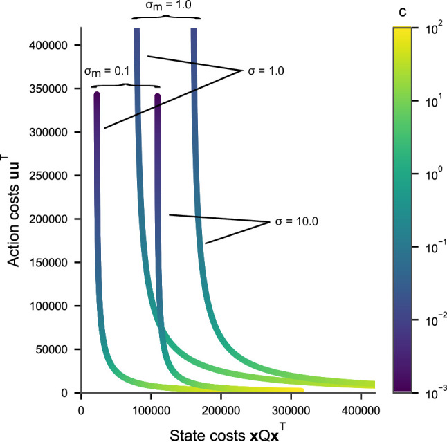
Figure 2—figure supplement 1. Pareto efficiency plot.

The Pareto efficiency plot visualizes the trade-off between two costs contributing to the cost function. The cost function is composed of two terms: state costs ${\displaystyle \mathbf{x}Q{\mathbf{x}}^T}$ and action costs ${\displaystyle \mathbf{u}{\mathbf{u}}^T}$, whose importance is balanced by the control cost parameter c. In a simulation, we computed these two terms separately for different values of c (see color bar) and plot them against each other. We did this for two levels each of action variability (${\sigma }_m$) and perceptual uncertainty (σ). First, there is a trade-off between tracking the target (state costs) and expending control effort (action costs): the better you track the target, the more action costs you have to tolerate. Second, the tracking performance depends on the values of the other two parameters: For a specific level of action variability ${\sigma }_m$ and perceptual uncertainty σ, there is a minimum level of state costs incurred, which cannot be alleviated by decreasing action costs via c.