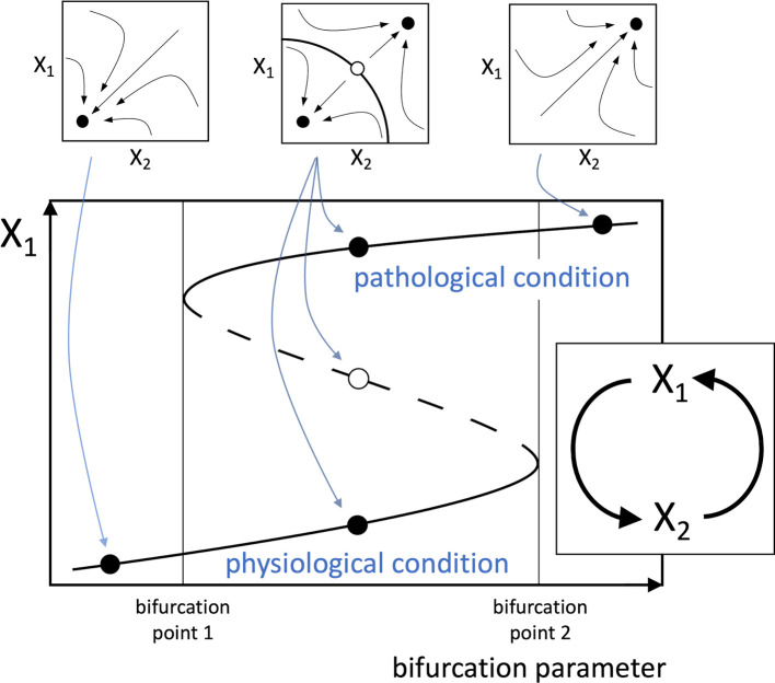
Figure 1. Schematic positive loop, representing a simplified model of a hypothetical pathogenic process.

The illustrated system captures the essential elements of the proposed theory, though more complex loops are likely to occur in real pathophysiological processes. The loop (inset below) consists of two functional agents, indicated by X ₁ and X ₂, which may represent the amounts or activities of cells (e.g. lymphocytes), enzymes (e.g. kinases), signal molecules (e.g. interleukins), etc. In the mathematical analysis of the loop, the dynamical interactions between the functional agents are described by a system of differential equations yielding the rate of change of the functional agents. In commonly used models of biological systems dynamics, each functional agent X _i is assumed to undergo spontaneous inactivation and evolve along time with time constant ${\mathrm{\tau }}_{{\mathrm{X}}_i}$ . The system of differential equations, in a schematic form, is the following:

$${\mathrm{\tau }}_{{\mathrm{X}}_1}{\dot{\mathrm{X}}}_1+{\mathrm{X}}_1=f\left({\mathrm{X}}_2\right)$$

$${\mathrm{\tau }}_{{\mathrm{X}}_2}{\dot{\mathrm{X}}}_2+{\mathrm{X}}_2=f\left({\mathrm{X}}_1\right)$$

A possible example for the functions appearing in the differential equations is the Hill function $f\left(\mathrm{x}\right)=\frac{\mathrm{\alpha }{x}^p}{1+\mathrm{\beta }{x}^p}$ , which is a suitable model for different stimulus-response relationships in biological systems ( Ferrante et al., 2009; Huang et al., 2014). However, f(X ₁) and f(X ₂) need not have the same form. By solving the system of differential equations, the trajectories followed by the system in the X ₁/X ₂ phase portrait can be traced (small plots at the top), showing the attraction basins of the stable equilibrium points (full dots), i.e. the system steady-states, and an unstable equilibrium point (empty dot). The bifurcation diagram (large plot below) shows the plot of the equilibrium values of X ₁ as a function of a bifurcation parameter, represented by one of the parameters of the differential equations. A similar plot can be derived for X ₂. The continuous lines represent stable equilibrium points and the dashed line unstable equilibrium points. As the bifurcation parameter increases (or decreases, depending on cases), the system can change from monostable (left), i.e. having a single stable equilibrium point, to bistable (middle), i.e. with two stable equilibrium points and an intermediate unstable equilibrium point, and eventually to monostable again (right). The two alternative stable equilibrium points represent the physiological and pathogenic conditions. Therefore, depending on the direction of variation, the bifurcation factor creates the conditions for the switch from physiological to pathogenic condition, or promotes the backward transition, respectively. The system also shows hysteresis, i.e. as shown in Figure 1, as the bifurcation parameter increases, and in the absence of other stimuli, the system is forced to abruptly jump from the physiological to the pathological condition at bifurcation point 2. However, once the system resides on the pathological condition, the reverse transition to physiological condition requires that the bifurcation parameter decreases until it reaches bifurcation point 1.