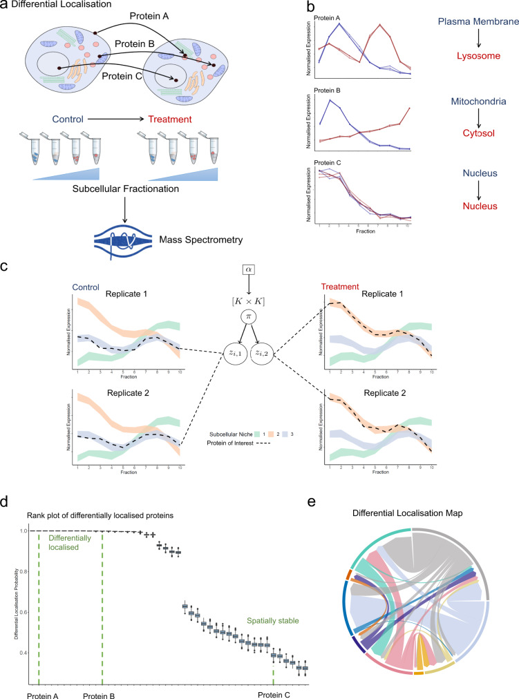
Fig. 1. An overview of the BANDLE workflow.
a A differential localisation experiment is set-up with a perturbation/treatment of interest. Orbitrap Image was generated by Fredrik Edfors at the Noun Project. b Mass-spectrometry-based spatial proteomics methods are applied to generate abundance profiles across the subcellular fraction. c BANDLE is applied by first calibrating the prior. The prior parameter is denoted by α. The model is visualised as follows: each dataset is described as a mixture of subcellular niches, modelled as Gaussian random fields. Allocations are obtained for each condition and then integrated between the two conditions, using a joint prior. π is a K × K matrix, where K is the number of subcellular niches analysed, where entry (j, h) is the probability that a protein is localised to niche j in the control and niche h in the treatment. zi,d is a categorical variable denoting the localisation of protein i in condition d. d The major results of BANDLE are represented in a rank plot. Sample size = 1000. Data are presented as medians with notches representing the interquartile range (IQR), and the whiskers extending to 1.5*IQR. e Example circos plot generated from the results of BANDLE. Source data are provided as a Source data file in the Supplementary material.

