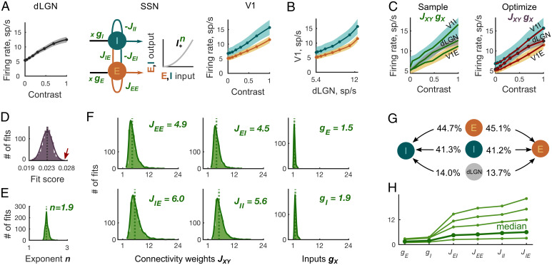
Fig. 3.

Inference of cortical and thalamic input weights from contrast responses using the SSN model. (A) The cortical network transforms the dLGN population contrast response (Left) to the contrast responses of E and I V1 populations (Right). The SSN model (Middle) represents the cortical network. The weights J_XY > 0 denote the strength of the recurrent connections from cortical population Y to X, and $g_X>0$ denotes the strength of the thalamic input to cortical population X. The transfer function relating input to output of the cortical E and I populations is $I_{+}^n={(\max \{I,0\})}^n$. Shaded areas represent ± SEM of the recorded responses. (B) Supralinear thalamocortical mapping of contrast responses excludes the exponent n = 1 in the SSN model. (C) (Left) Randomly generated sample curves (green lines) within ± SEM of the dLGN and V1 contrast responses (shaded areas) were substituted into the SSN model to yield the initial parameters J_XY and g_X for the fixed exponents n. (Right) Subsequently, the SSN parameters J_XY, g_X, and n were optimized to minimize the distance between the fit (red) and the mean of the recorded responses (orange, gray, and teal). (D) The distribution of fit scores of the final 10³ fits has a mean of $2\times {10}^{-2}$. The arrow (red) points to the largest score value used to produce the example fit in C (red). (E) The distribution of the optimized power law exponents n corresponding to the final 10³ fits has a median of n = 1.9. (F) The distributions of the optimized connectivity weights J_XY are broader than that of input weights g_X. The location of vertical dotted lines corresponds to the J_XY and g_X medians presented in the plot’s upper right corners. (G) The average ratios of connectivity weights from three input sources (local E, local I, and external dLGN) to E cortical population are similar to those to the I population. (H) In 99% of the inferred connectivity parameter sets, the recurrent and input connectivity weights, ordered according to the x axis labels, build an increasing sequence. Thin green lines indicate four representative examples of fits; bold green line indicates median of parameter distributions.