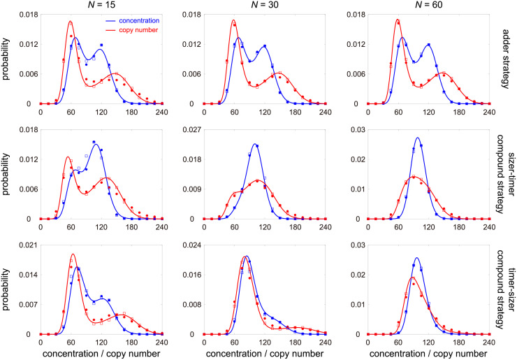
Fig 3. Comparison between the full and mean-field models under different choices of N and different size control strategies.

The blue (red) dots show the simulated concentration (copy number) distribution for the full model obtained from the stochastic simulation algorithm (SSA). The blue (red) squares show the simulated concentration (copy number) distribution for the mean-field model obtained from SSA. The blue (red) curve shows the analytical approximate concentration (copy number) distribution given in Eq (8) (Eq (15)). The full and mean-field models are in good agreement when N ≥ 15 and they become almost indistinguishable when N ≥ 30. Moreover, the analytical solution performs well when N ≥ 15 and perform excellently when N ≥ 30. The model parameters are chosen as N₀ = 0.4N, B = 1, β = 0, κ = 2, d = 1, η = 10, where η = d/f is the ratio of the degradation rate to cell cycle frequency. The growth rate g is determined so that f = 0.1. The parameters ρ and a are chosen so that the mean gene product number 〈n〉 = 100 and the mean cell volume 〈V〉 = 1. The strengths of size control are chosen as α₀ = α₁ = 1 for the upper panel, α₀ = 2, α₁ = 0.5 for the middle panel, and α₀ = 0.5, α₁ = 2 for the lower panel. When performing SSA, the maximum simulation time for each lineage is chosen to be 10⁵. To deal with the time-dependent propensities in the full model, we use the numerical algorithm described in [85, Sec. 5].