Fig. 5. Evolutionary history of the inversion.

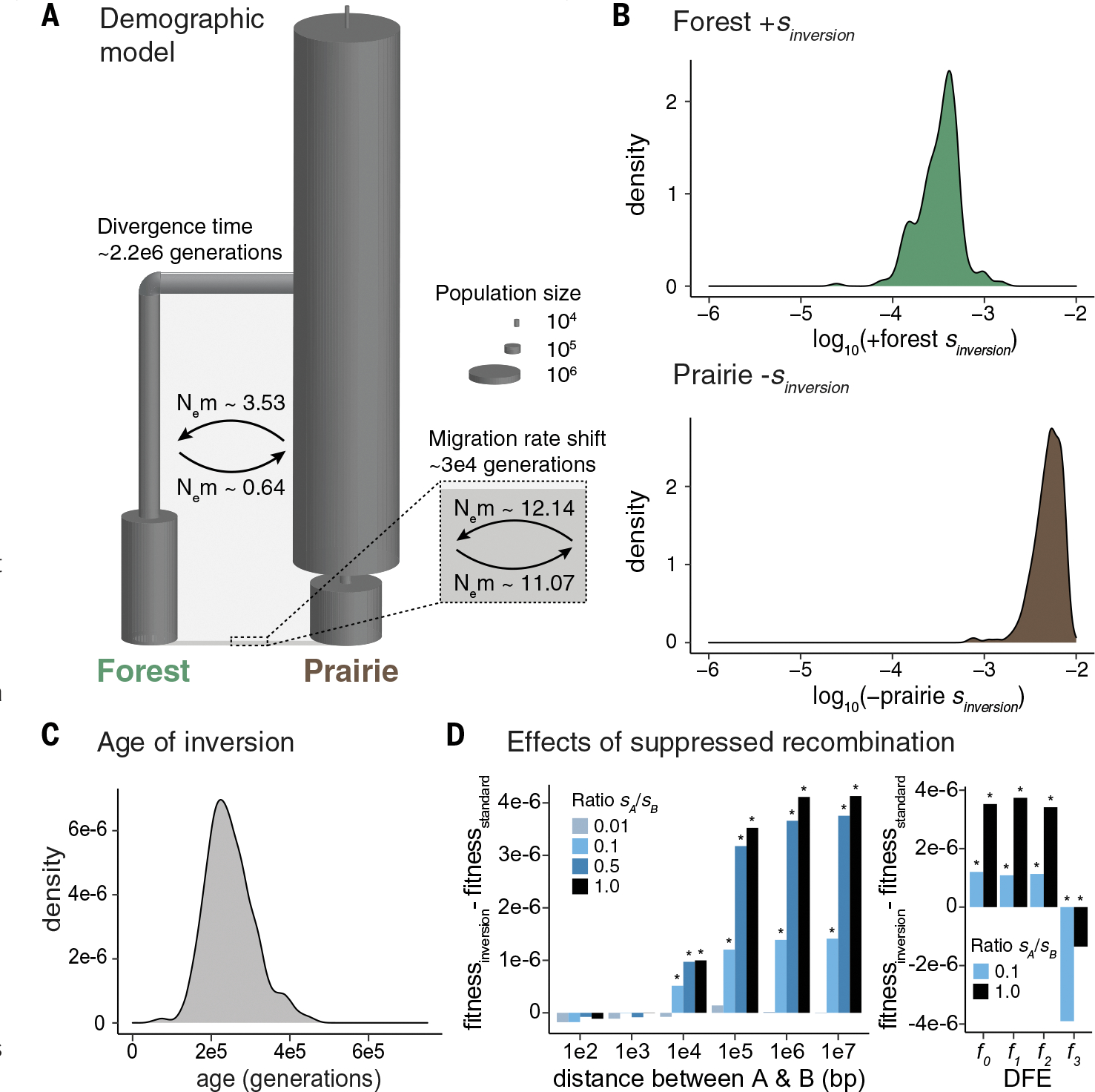
(A) Best-fit demographic model. N_e, effective population size; m, migration rate. (B) Posterior probability distributions for the selection coefficient associated with the inversion in the forest (top, green) and prairie (bottom, brown) populations, when the inversion is introduced 150,000 generations ago (for additional introduction times, see fig. S13). The estimated selection coefficient is positive in forest and negative in prairie. (C) Posterior probability distribution for the age of the inversion. (D) Estimated fitness effects of suppressed recombination within the inversion. Two beneficial loci (A and B) were introduced into the forest population on the inversion or on a standard haplotype, varying the ratio of the selection coefficients for A (s_A) and B (s_B), with s_A + s_B kept constant at 3 × 10⁻⁴. bp, base pairs. Bar height shows the difference in final mean fitness of the forest population between the inversion and standard haplotype scenarios. Asterisks indicate a significant difference in mean fitness (P < 0.05) computed with permutation tests. (Left) Two beneficial loci at varying distances apart, without deleterious mutations. (Right) Two beneficial loci separated by 100 kb, with deleterious mutations introduced according to distributions of fitness effects (DFE): f₀: 100% of mutations neutral (2Ns = 0, where N indicates population size and s indicates selection coefficient); f₁: 50% of mutations neutral (2Ns = 0), 50% weakly deleterious (−10 < 2Ns < −1); f₂: 33% of mutations neutral (2Ns = 0), 33% weakly deleterious (−10 < 2Ns < −1), 33% moderately deleterious (−100 < 2Ns < −10); f₄: 25% of mutations neutral (2Ns = 0), 25% weakly deleterious (−10 < 2Ns < −1), 25% moderately deleterious (−100 < 2Ns < −10), 25% strongly deleterious (−1000 < 2Ns < −100).