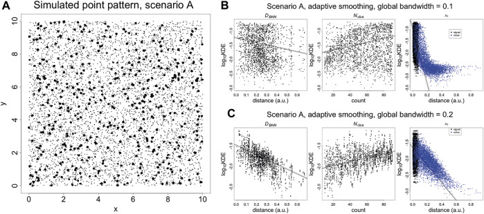
FIGURE 2.
(A) Simulated SMLM image of spatially random molecules. Molecules are generated using a Poisson process with intensity of five over a square window with sides of length 10 (arbitrary units). The molecules are replaced with clusters of localisations, generated with a bivariate normal distribution with variance of 0.000625 and covariance of zero. The number of localisations per cluster is an integer randomly sampled on the interval (10, 90). Finally, the noise localisations are generated using a Poisson process with intensity of 50. D B , D BNN , N clus plotted vs Kernel Density Estimates (KDE). (B) KDE (adaptive smoothing) of Figure 4 fitted with a global bandwidth of 0.1. (C) KDE (adaptive smoothing) of Figure 4 fitted with a global bandwidth of 0.2. At low values of the bandwidth, it is possible to differentiate between signal and noise localisations but the trend with D BNN and N clus becomes less clear. At a higher value of the bandwidth, the trend D BNN and N clus becomes clear but it is no longer possible to differentiate between signal and noise localisations. This highlights that a KDE at using a single bandwidth is not adequate to capture the entire spatial structure. Trend lines are fitted with a linear model and are supplied for visualisation purposes.

