Evaluating and Modeling Neighborhood Diversity and Health Using Electronic Health Records

Abstract

Background:

Electronic health records (EHRs) provide researchers with abundant sample sizes, detailed clinical data and other advantages for performing high-quality observational health research on diverse populations. We review and demonstrate strategies for the design and analysis of cohort studies on neighborhood diversity and health, including evaluation of the effects of race, ethnicity and neighborhood socioeconomic position (SEP) on disease prevalence and health outcomes, using localized EHR data.

Methods:

Design strategies include integrating and harmonizing EHR data across multiple local health systems and defining the population(s) of interest and cohort extraction procedures for a given analysis based on the goal(s) of the study. Analysis strategies address inferential goals, including the mechanistic study of social risks, statistical adjustment for differences in distributions of social and neighborhood-level characteristics between available EHR data and the underlying local population, and inference on individual neighborhoods. We provide analyses of local variation in mortality rates within Cuyahoga County, Ohio.

Results:

When the goal of the analysis is to adjust EHR samples to be more representative of local populations, sampling and weighting are effective. Causal mediation analysis can inform effects of racism (through racial residential segregation) on health outcomes. Spatial analysis is appealing for large-scale EHR data as a means for studying heterogeneity among neighborhoods even at a given level of overall neighborhood disadvantage.

Conclusions:

The methods described are a starting point for robust EHR-derived cohort analysis of diverse populations. The methods offer opportunities for researchers to pursue detailed analyses of current and historical underlying circumstances of social policy and inequality. Investigators can employ combinations of these methods to achieve greater robustness of results.

Socioeconomic conditions broadly and strongly influence health status and health outcomes.^1–3 In the United States and elsewhere, racism and adverse socioeconomic conditions can impose vulnerabilities that result in routinely unmeasured baseline risks of disease and variation in care quality. Earlier this year, MDM released a policy statement on the use of demographic classification variables that established a requirement for authors to “clearly define 1) what they believe the variables are measuring and 2) what hypotheses or research questions justify the inclusion of these variables in the analysis or model.”⁴

Social and economic mechanisms⁵ such as insufficient access to health insurance and health care appointments; structural and/or interpersonal racism; differential access to healthful foods and locations for safe physical activity and social connectedness; and differential exposure to pollutants lead to disparities in timely disease identification and treatment and in subsequent outcomes. Rooted in generations of state and local laws enforcing racial segregation, racist lending policies and systematic disinvestment have led to residential segregation in many U.S. cities, systematically disadvantaging Black, Hispanic and other marginalized racial and ethnic groups and imposing or exacerbating severe neighborhood-level health inequities.⁶ Global health researchers (such as Paul Farmer) have long highlighted the challenges in providing care across varied cultural and socioeconomic conditions, and the need for tailored local approaches. Thus, to develop effective approaches to community-specific health problems we must use data and modeling approaches that properly account for local contexts.⁷

Place-based health inequities, which are embedded within everyday care, can impact long-term patient health outcomes. In a prior study, Dalton et al. determined that cardiovascular risk in Northeast Ohio is more strongly related to characteristics of neighborhoods than to traditional clinical risk measures (although both types of risk assessment contributed).⁸ The ability of widely relied upon risk assessment tools (specifically the Pooled Cohort Equations⁹) to accurately depict risk levels varied strongly with neighborhood socioeconomic position (SEP). In this context, conjectures about why such heterogeneity exists include potential exposures (e.g. air pollution, stress), poverty, and subgroup characteristics (such as differences in epigenetic alterations) that are primarily present among persons from lower resourced neighborhoods.^10,11 Recognizing and pursuing the sources of risk and outcome heterogeneity are essential first steps in seeking and understanding the mechanisms responsible for differences in health status and health outcomes.

Electronic health records (EHRs) are an ample scientific resource for investigating the complexity of social and place-based inequities in health status, care and outcomes, within and among diverse, socially-defined subpopulations.¹² In this paper, we review and demonstrate both design and analysis approaches to studying the effects of race, ethnicity and neighborhood socioeconomic position (SEP) on disease prevalence and health outcomes using localized EHR data. We illustrate these strategies through an analysis of regional EHR data from Northeast Ohio and discuss the relative advantages of each approach as well as ways in which approaches might be combined in practice.

Design Considerations

Cohort Identification and Extraction

Health systems serve specific patient populations that are largely determined by geography and market dynamics. Contracts with insurers and competition lead to selection of distinct patient populations for each system.¹³ Furthermore, as insurance plans differ in the degree and nature of coverage for health services, health systems can systematically vary practice patterns, leading to neighborhood and socioeconomic differences in disease prevalence; administered treatments and their timing; and outcomes. Likewise, there is significant neighborhood-level variability in overall insurance rates, choice (or lack thereof) of individual insurance plans, and health care utilization patterns.

These concerns must be carefully considered in designing studies of neighborhood diversity and health. Investigators must consider the racial, ethnic and socioeconomic distribution of the patient populations represented in a given system, which can significantly depart from those of local populations. The fundamental design consideration of what defines the population(s) of interest for inference is critical in determining the type of analyses to be done. In observational clinical research, investigators traditionally hypothesize singular, average treatment effects and may or may not secondarily evaluate effect heterogeneity (typically, through estimation of subgroup or interaction effects). In diverse populations (especially those with varied baseline risk of outcomes), estimates of average treatment effects can be biased.¹⁴

Here, we introduce our first strategy for more robust inference: Combining EHR data across health systems within a region can improve alignment in demographic and socioeconomic characteristics between the source data and the regional population. In Northeast Ohio, two of the largest health systems are Cleveland Clinic Health System (CCHS) and MetroHealth System (MHS). CCHS consists of a large regional network of hospitals and outpatient facilities. Its patient population is substantial and consists of a relatively large proportion of privately-insured and Medicare patients. MHS is the region’s predominant safety net system, comprising a network of hospitals and outpatient facilities. The two care systems often share resources and patients, but there are differences in the characteristics of the patient populations, notably that MHS cares for a relatively large proportion of patients covered by Medicaid and persons from lower-resource communities.

The NEOCARE Learning Health Registry combines up to 22 years of EHR data for 3.1 million unique individuals residing in Northeast Ohio and being seen at either CCHS or MHS (approximately 70% of the local population of adults). We linked and de-duplicated data across institutions using an IRB-approved algorithm based on shared individual identifiers; that is, records at CCHS and MHS for persons who encountered care at both system were harmonized and assigned to a single, anonymized NEOCARE study identifier. The NEOCARE registry is maintained in CCHS’s Department of Quantitative Health Sciences via a Data Transfer Agreement between MHS and CCHS. Inclusion criteria for the registry are broad, such that analytic cohorts for individual studies can be effectively extracted: Patients are included in the registry if they have a history of 2 or more documented outpatient (either specialty or non-specialty) visits at either CCHS or MHS. Mortality data are obtained from multiple sources, including the EHR itself, the Ohio Department of Health Vital Statistics and the Social Security Death Master File (for deaths prior to 2011). Further details of the NEOCARE Learning Health Registry are described in Taksler et al. (2020).¹²

Geocoding and Integration with Neighborhood Data Sources

Residential addresses that are stored in EHR data are critical for facilitating analyses of place-based health disparities. Examples of public and private neighborhood environmental data sources include the American Community Survey, U.S. Department of Agriculture Quick Stats, EnviroAtlas (from the U.S. Environmental Protection Agency), U.S. Bureau of Labor Statistics Public Data Application Programming Interface, and New York University’s City Health Dashboard¹⁵. Commonly, these data sources are area-referenced according to U.S. Census block groups or tracts.

The process of geocoding patient addresses in the EHR into Census-designated areas has been described elsewhere.¹⁶ In the NEOCARE registry, residential location history of each patient included is geocoded to latitude and longitude, spatially-joined with Census TIGER/Line shapefiles to associate residential locations with their corresponding Census blocks, and linked to these data sources at the highest spatial resolution available (typically, at the census block group level).

Demonstration: Analysis of Local Mortality Patterns Among Older Adults in Cuyahoga County, Ohio

To assist in our presentation of the methodological approaches being described herein, we conducted a variety of analyses of socioeconomic and neighborhood-level variability in all-cause mortality risk among older adults. These analyses are demonstrative: a full treatment of the topic is outside the scope of this paper.

We extracted from the NEOCARE registry a cohort of patients aged ≥ 60 years whose EHR-documented race and ethnicity was Non-Hispanic (NH) Black, NH white, Hispanic or Asian. We restricted analyses to these racial and ethnic groups because other groups were too sparsely represented among our two health systems for robust inference. For each patient, the first observed outpatient visit (primary care, geriatrics, specialty visits, etc.) after turning age 60 was used as the index (or baseline) visit. We included patients whose index visit occurred between 2005 and 2015; whose geocoded address of residence for this index visit was located in Cuyahoga County, Ohio; and who had at least one visit (or died) within 2 years after the index visit.

Neighborhood socioeconomic position corresponding to patients’ geocoded addresses of residence was characterized using the 2015 Ohio Area Deprivation Index (ADI). We used the sociome R package¹⁷ to estimate 2015 Ohio ADI values, using American Community Survey 5-year estimates at the census block group level. The sociome package replicates the methodology of Kind et al.¹⁸ for user-defined reference regions, such that factor loadings and index values are normalized to the region of interest (as opposed to the entire country). Details are provided elsewhere.^17–20 For most analyses, we analyzed ADI values based on quintiles of the distribution among Ohio block groups: ADI quintile 1 corresponded to the lowest level of neighborhood socioeconomic deprivation, while ADI quintile 5 corresponded to the highest level of neighborhood socioeconomic deprivation. However, for our spatial analysis, we used (continuous) ADI values.

Our analytic cohort included 38,042 patients whose index encounter occurred at MHS and 177,255 patients whose index encounter occurred at CCHS, for a total of 215,297 patients. Figure 1 describes the distributions of race and ethnicity and ADI quintiles for adults over age 60 in each health system as well as in the combined NEOCARE cohort. Compared to the county population of adults over age 60, MHS patients tended to be disproportionately from lower-resourced (higher ADI) neighborhoods and disproportionately non-Hispanic Black, Hispanic and Asian. The racial and ethnic distribution for CCHS patients was generally similar to that of the county population, while the socioeconomic distribution skewed toward higher socioeconomic position (lower-ADI quintiles). The combined NEOCARE cohort including data from both health systems more closely matched that of the county population.

Figure 1/.

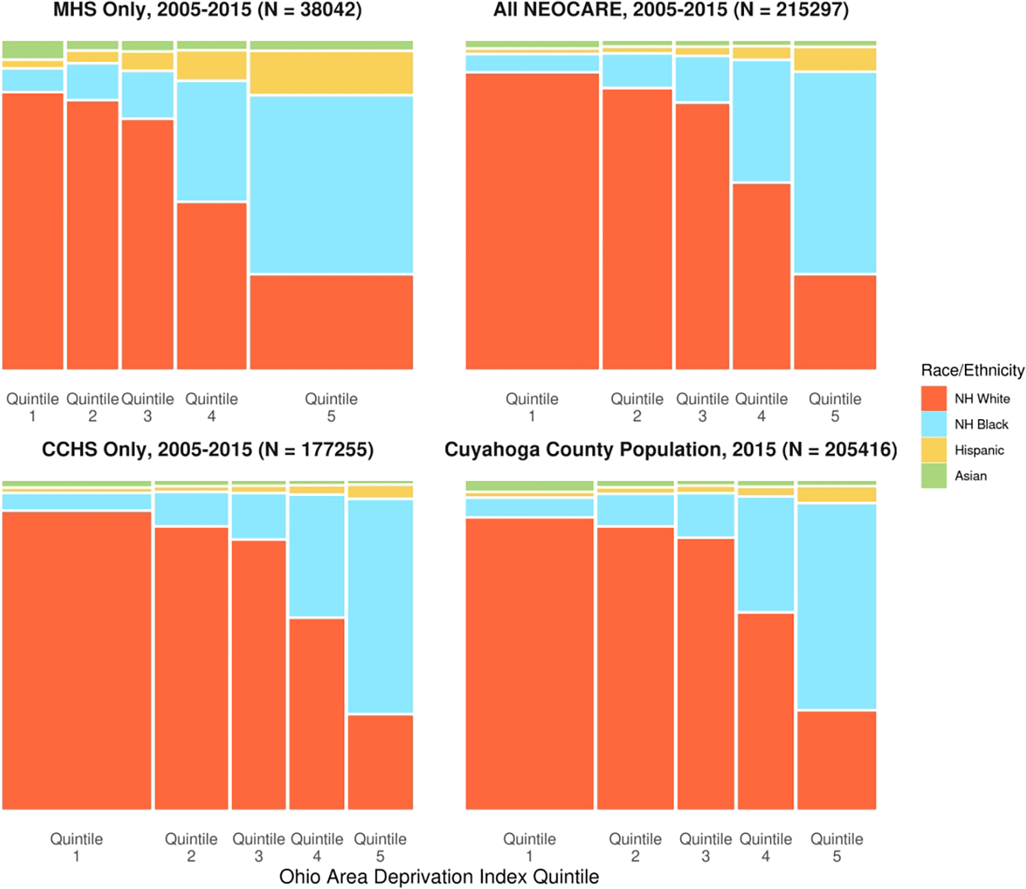
Mosaic plots of the joint distribution of race and ethnicity and Ohio Area Deprivation Index quintile for MHS patients aged ≥ 60 years who resided in Cuyahoga County, Ohio and who were seen between 2005 and 2015; for CCHS patients meeting the same criteria; for the combined NEOCARE cohort; and for the population of adults aged ≥ 60 years residing in Cuyahoga County, Ohio in 2015. Bar widths reflect the proportion of a residents from communities in a given ADI quintile within a sample (or within the county population). ADI quintiles 1 and 5 represent the least and most socioeconomically disadvantaged quintiles, respectively.

Analysis Considerations

Unweighted Analysis of the Entire Cohort

When data integration leads to samples in balance with underlying socially-defined populations, analyses of the unweighted cohort may be considered. To demonstrate this, we modeled mortality rates as a function of age, sex, race, ethnicity and ADI quintile using a Poisson rate model (number of deaths per 100 person years). Of interest were i) ratios of mortality rates among racial and ethnic groups, ii) rate ratios among ADI quintiles, and iii) the mediating effect of ADI quintile on the relationship between race and ethnicity and mortality (race and ethnicity → ADI quintile → mortality). An informal way to evaluate this mediating effect is by fitting two models, with the first including age, sex and racial and ethnic group as predictors and the second adding ADI quintile; comparisons of rate ratios associated with racial and ethnic groups between these two models can inform the degree of the association accounted for by ADI quintile. More formally, we quantified the percentage of racial and ethnic disparities (log rate ratios) accounted for by ADI via causal mediation analysis methods. For this purpose, we used the mediate R package.²¹

Table 1 contains age- and sex-adjusted incidence rate ratios (IRRs) and 95% confidence intervals (CIs) comparing non-Hispanic Black, Hispanic and Asian patients to non-Hispanic white patients, both before and after adjustment for ADI quintile. Prior to adjustment, non-Hispanic Black patients had a significantly higher mortality rate (IRR [95% CI]: 1.31 [1.28 – 1.34]); the relationship was not significant after adjustment for ADI quintile (IRR [95% CI]: 1.02 [0.99 – 1.05]). Compared to non-Hispanic white patients, the reductions in mortality rates for Hispanic and Asian patients were more pronounced after adjusting for ADI. Causal mediation analysis indicated that ADI (as a continuous variable) accounted for 113% of the elevated mortality risk (average proportion mediated [95% CI]: 1.13 [1.02 – 1.26]) for non-Hispanic Black patients compared to non-Hispanic White patients.¹

Table 1.

Age- and sex-adjusted incidence rate ratios for mortality comparing Non-Hispanic (NH) Black, Hispanic and Asian patients to NH White patients, without and with adjustment for Area Deprivation Index (ADI) quintile (1 = least socioeconomic disadvantage; 5 = highest socioeconomic disadvantage).

	Model 1 Age, Sex, Race and Ethnicity			Model 2 Age, Sex, Race, Ethnicity, and ADI Quintile
	IRR1	95% CI1	p-value	IRR1	95% CI1	p-value
Race and Ethnicity
NH White	—	—		—	—
NH Black	1.31	1.28, 1.34	<0.001	1.02	0.99, 1.05	0.2
Hispanic	0.84	0.77, 0.90	<0.001	0.67	0.61, 0.72	<0.001
Asian	0.48	0.42, 0.55	<0.001	0.46	0.40, 0.52	<0.001
ADI Quintile
Quintile 1				—	—
Quintile 2				1.31	1.27, 1.35	<0.001
Quintile 3				1.46	1.41, 1.50	<0.001
Quintile 4				1.58	1.53, 1.63	<0.001
Quintile 5				1.78	1.72, 1.84	<0.001

¹IRR = Incidence Rate Ratio, CI = Confidence Interval

Sampling and Weighting

EHR data are massive, and, for many questions, might be described as substantially “overpowered”. When the goal of the analysis is to make single-population inferences and socio-demographic characteristics are not of primary interest, sampling or weighting approaches can be considered as a strategy to make more robust and representative inferences on the (single) underlying local population. Here, we will focus on robust estimation of age-specific mortality rates in Cuyahoga County, Ohio and adjust our estimates for differences in distributions of race, ethnicity and ADI quintile between NEOCARE data and the population of Cuyahoga County adults aged ≥ 60 years.

Consider the comparison of race and ethnicity across ADI quintile distributions between those included in the NEOCARE registry compared to the general Cuyahoga County population. Let n_ij and p_ij represent, respectively, the number and proportion of observations in the available EHR cohort (in our case, the combined NEOCARE sample) for racial/ethnic group i and ADI quintile j. Let q_ij represent comparable proportions of race and ethnicity and ADI quintile groups in the population of adults aged ≥ 60 years residing in Cuyahoga County, and define a sampling ratio, i.e., a measure of the extent to which each group is over- or under-represented in the data, as R_ij = p_ij/q_ij. Here, we will reduce sample sizes in all but the most under-represented group so that the distributions of race and ethnicity and ADI quintile in the resulting sample match the distributions in the referent population. Let this minimum value be R * = min (R_ij), the number of sampled patients in this group be n * and the proportion of the target population who are members of this group be q *.

Table 2 includes these quantities for our demonstration study. The most under-represented group in NEOCARE was Asian patients from neighborhoods in the 1^st ADI quintile (n * = 1,337; 0.0062 of NEOCARE patients vs. 0.0093 of the Cuyahoga County population aged ≥ 60 years; R * = 0.667). Prior to sampling, the total NEOCARE sample size was 215,297. As our sampled data must include a proportion of 0.0093 for this most under-represented group, we can calculate the size of the sampled data as the number of available patients in this group divided by this proportion, i.e., n′ = n * /q * = 1,337/0.0093 = 143,763. This leads to group-specific sample sizes of $n_{ij}^{\prime }=n^{\prime }\left(q_{ij}\right)$ and group-specific sampling weights of ${\varphi }_{ij}=n_{ij}^{\prime }/n_{ij}$. For Asian patients from neighborhoods in the 1^st ADI quintile, the process yielded $n_{ij}^{\prime }=1337$ and ϕ_ij = 1.0 (since it was the most under-represented group).

Table 2.

Quantities derived via sampling and weighting from the combined NEOCARE cohort and Cuyahoga County population. Groups were defined on the basis of race, ethnicity and Area Deprivation Index (ADI) quintile. For the sampling approach, the observed group-specific samples (of original size n_ij and proportion p_ij) are randomly sampled with frequencies φ_ij to result in the sampled group sizes $n_{ij}^{\prime }$ that are proportional to the population frequencies (q_ij) and of size that is determined by the extent of under-representation in the sample (minimum sampleto-population ratio R_ij, in bold and italic). For weighting, all observations are used but case weights of w_ij are applied such that each group’s weighted sample size w_ijn_ij is similarly proportional to q_ij. ADI quintiles 1 and 5 represent the least and most socioeconomically disadvantaged quintiles, respectively.

Race and Ethnicity	ADI Quintile	nij	pij	qij	Rij	φij	$n_{ij}^{\prime }$	wij	wijnij
NH White	Quintile 1	67319	0.313	0.295	1.060	0.630	42410	0.943	63508.5
	Quintile 2	33086	0.154	0.171	0.901	0.741	24526	1.110	36724.0
	Quintile 3	24139	0.112	0.121	0.925	0.722	17424	1.081	26098.5
	Quintile 4	18120	0.084	0.087	0.973	0.686	12436	1.027	18615.0
	Quintile 5	13109	0.061	0.061	1.002	0.667	8741	0.998	13087.5
NH Black	Quintile 1	3421	0.016	0.017	0.952	0.702	2401	1.050	3593.1
	Quintile 2	3724	0.017	0.018	0.972	0.687	2559	1.029	3831.6
	Quintile 3	3957	0.018	0.019	0.995	0.672	2660	1.005	3978.5
	Quintile 4	11708	0.054	0.050	1.090	0.613	7174	0.917	10739.5
	Quintile 5	27942	0.130	0.127	1.020	0.654	18287	0.980	27382.3
Hispanic	Quintile 1	563	0.003	0.003	0.929	0.716	403	1.077	606.3
	Quintile 2	434	0.002	0.002	0.952	0.696	302	1.050	455.7
	Quintile 3	565	0.003	0.002	1.300	0.510	288	0.769	434.6
	Quintile 4	1044	0.005	0.003	1.655	0.399	417	0.604	630.8
	Quintile 5	3052	0.014	0.009	1.632	0.410	1251	0.613	1869.9
Asian	Quintile 1	1337	0.006	0.009	0.667	1.000	1337	1.500	2005.5
	Quintile 2	468	0.002	0.003	0.786	0.861	403	1.273	595.6
	Quintile 3	370	0.002	0.001	1.308	0.505	187	0.765	282.9
	Quintile 4	354	0.002	0.002	0.889	0.732	259	1.125	398.2
	Quintile 5	585	0.003	0.002	1.286	0.516	302	0.778	455.0

Sampling approaches inherently discard data, which may be undesirable. Weighting methods avert the need to discard observations altogether by correcting any existing imbalances between a sample and the population. Continuing our example above, weighting each group according to the ratio of the proportion in the population to the proportion in the sample (i.e., $w_{ij}=R_{ij}^{-1}=q_{ij}/p_{ij}$) results in a weighted sample with group sizes proportional to those in the population (i.e., w_ijn_ij ∝ q_ij). See Table 2. For Asian patients from neighborhoods in the 1^st ADI quintile, we had w_ij = 1.5 and w_ijn_ij = 2005.5.

Sampling and weighting methods are flexible and can be extended or generalized to any chosen set of variables the investigator desires to use to balance their sample against any chosen reference population. Our examples were performed at the group level; these methods can be straightforwardly applied at the observation level, allowing greater flexibility in defining observation-specific sampling probabilities and weights. For example, the group-specific sampling weights ϕ_ij and the case weights w_ij can be directly applied at the individual level after matching the weights to each case based on group membership. Alternatively, weights that are a function of both continuous and discrete variables can be defined from individual-level data via logistic regression models; interested readers are referred to the literature on inverse probability weighting.^22,23

These approaches could similarly be used to reflect the broader U.S. population. For instance, in Cuyahoga County we have fewer Hispanic and Asian individuals than the rest of the United States. Instead of using reference proportions (q_ij) based on the local population of Cuyahoga County residents, one might consider sampling or weighting the data using reference proportions from the entire country (or other regions). However, these techniques have an important limitation to consider in that they are based on an assumption (which rarely if ever holds in the real-world) that local health outcomes are generalizable to other or broader populations that age, grow and develop under different health systems and environmental conditions. As such, one may consider using the unweighted estimates in the sample as a representation of minority/disadvantaged populations at particular local institutions as opposed to weighted estimates in an attempt to possibly fail to generalize to broader geographical regions.

Figure 2 displays sex-specific estimates of death rates (per 100 person-years) as a function of age for i) health system-specific populations and ii) the Cuyahoga County population (via sampling and weighting, respectively). Sampling and weighting approaches resulted in similar point estimates for both males and females. No notable differences in the relationship were observed for females when estimating the model using the various approaches; however, for males, single-system estimation of the relationship produced a curve that was as much as 20% different from those estimated for the Cuyahoga County population via sampling or weighting.

Figure 2/.

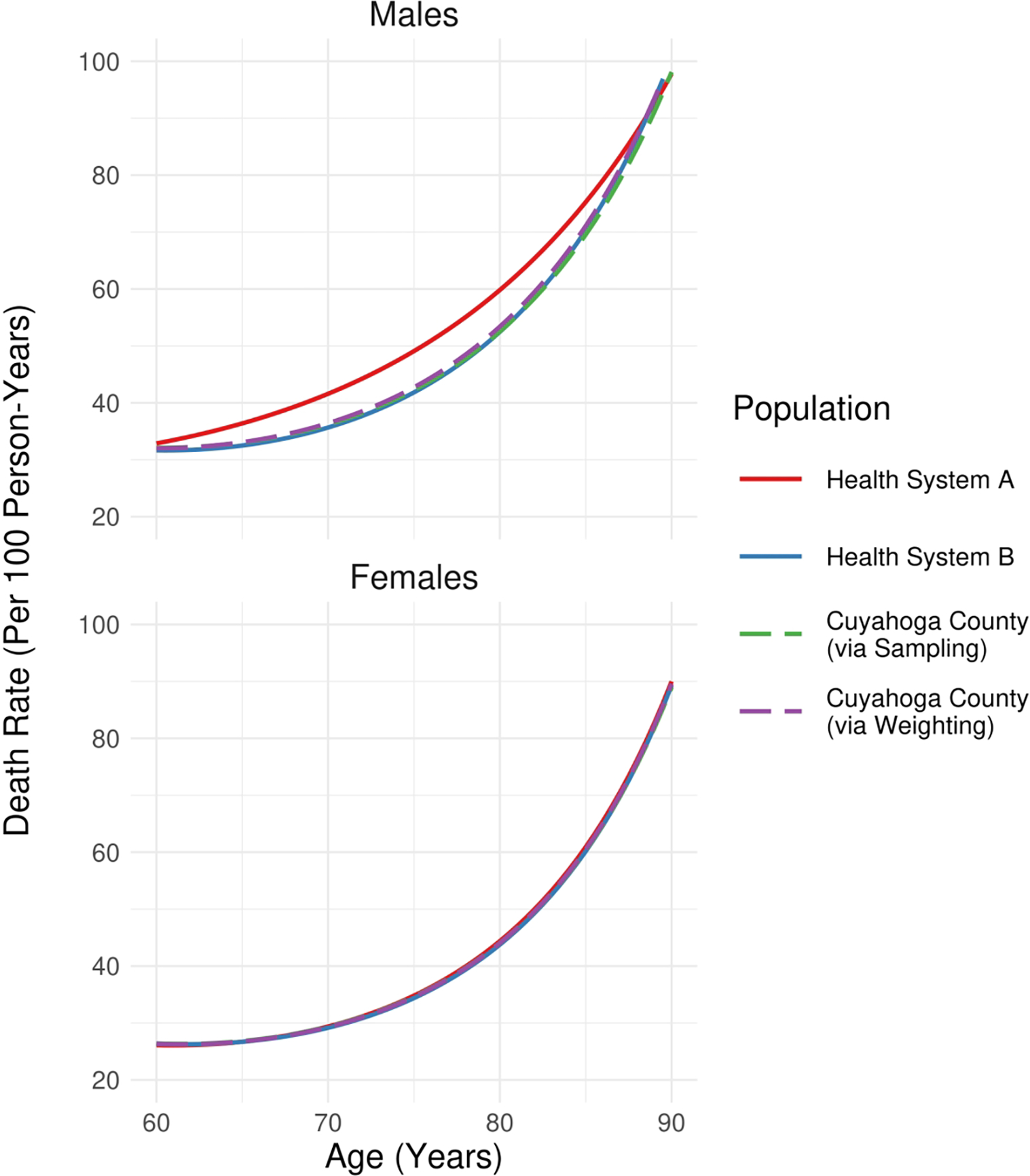
Estimates of death rates per 100 person-years for health system-specific populations as well as those of the population of Cuyahoga County residents aged ≥ 60 years (via sampling or weighting of the NEOCARE registry to align socio-demographic characteristics of the data with those of the underlying population). Health system identities are redacted for this illustrative analysis.

Stratification

Sampling and weighting are intended to produce more representative population-level estimates that account for imbalances between sampled data and population characteristics. In particular, these approaches evaluate sex, race, ethnicity and neighborhood deprivation marginally. This is inconsistent with frameworks of intersectionality where overlapping social, political and economic identities of subpopulations generate numerously unique experiences of disadvantage and oppression.²⁴ Results may be distinct among, for example, Non-Hispanic Black males in a specific neighborhood (intersectionally-defined group) in relation to i) Non-Hispanic Black persons, ii) males or iii) residents of that neighborhood (marginally-defined groups). Stratification is frequently necessary – at the very least as a sensitivity analysis – to understand heterogeneous effects in diverse, intersectional patient populations. In EHR studies with very large sample sizes (often reaching into the thousands, even for proportionally smaller subgroups), stratification is a more viable strategy than in many other data contexts. Stratified estimates may be obtained either by incorporating interaction effects or by directly subsetting the dataset according to pre-defined groups. Even when conducting a stratified analysis, sampling and weighting approaches should be considered, especially in situations where only a subset of social characteristics are being used to define strata.

Stratification can be readily achieved with modern data science toolkits. For example, the nest_by and mutate functions in the dplyr R package²⁵ can be used to stratify a dataset by a selected set of grouping factors and estimate separate regression models for each strata in two lines of code. A comparable technique for considering heterogeneous effects among subgroups is to incorporate interaction terms in a model involving the whole dataset; however, it is to be noted that the nature of covariate adjustment is different when employing the interaction approach. That is, estimates are adjusted to fixed and arbitrary values over the entire population of interest as opposed to values among a specific subpopulation.

Stratification also encourages analysts to consider whether the populations of interest are all adequately represented in terms of available sample sizes for analysis. For example, our analytic cohort included 5,658 Hispanic patients and 3,114 Asian patients. Here and in other studies, the ability to make inferences by stratification, particularly for those representing smaller percentages of the underlying population, is dependent on outcome rates and the distribution of other stratifying concepts (here, the regional distribution of patients across neighborhood socioeconomic categories).

These limitations are borne out in the analysis presented in Figure 3. We separately estimated mortality rates and 95% confidence intervals for groups defined on the basis of sex, race, ethnicity and ADI quintile (Quintiles 1–2 and 3–4 were grouped together for this analysis). Estimates for Asians were unreliable due to small sample sizes. Confidence intervals for Hispanic groups were wider than those for Non-Hispanic Blacks and Non-Hispanic Whites. Likewise, confidence intervals for adults over age 80 who resided in low-resource (Quintile 5) neighborhoods were wide since that age range is in many cases well beyond the life expectancy observed in such neighborhoods.

Figure 3/.

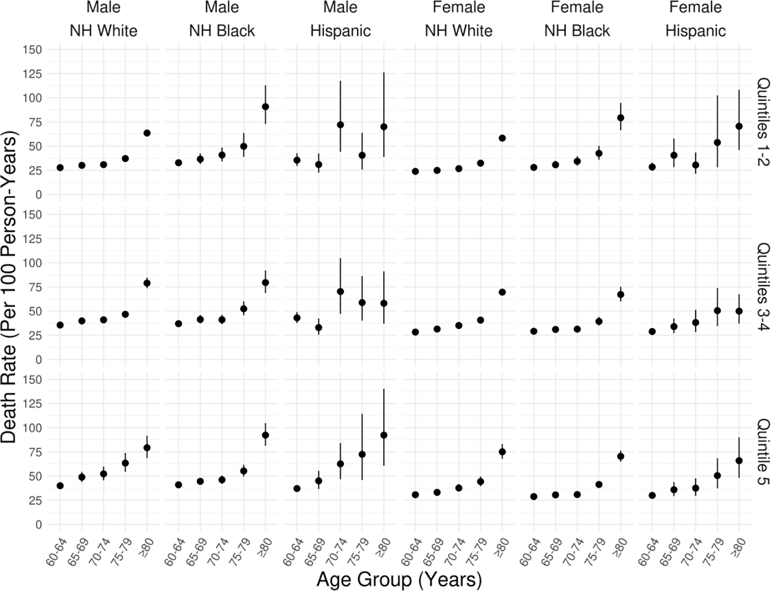
Stratified estimates of death rates (per 100 person-years) by sex, race, ethnicity and ADI quintile obtained the NEOCARE registry. Each panel in the figure represents a subpopulation defined by these characteristics (race and ethnicity define the columns and ADI quintile groupings define the rows). Sample sizes for Asians were insufficient for reliable estimation. ADI quintiles 1 and 5 represent the least and most socioeconomically disadvantaged quintiles, respectively.

Mapping and Spatial Analysis

The above approaches are aspatial. In large-scale studies where neighborhood-level diversity is of interest, mapping and spatial analysis methods should be used. In particular, the manifestations of neighborhood socioeconomic deprivation are themselves diverse, and, by extension socio-ecological mechanisms underlying health disparities may differentially impact some low-SEP neighborhoods more than other low-SEP neighborhoods. This leads to hypotheses of local patterns of health disparity.

Spatial analysis methods can identify areas where health outcomes are worse (e.g., “hotspots”); understand the relationships between neighborhood-level characteristics and health outcomes; and decompose neighborhood-level variation in health outcomes. Note that ADI provides a composite measure of neighborhood status and neighborhoods with different characteristics may have the same ADI value; this is true of many area-based indicators. Thus, spatial analysis provides a key strategy to evaluate health outcomes among socio-economically disadvantaged and racially diverse neighborhoods when coupled with EHR data.

The EHR is an abundant source of medical data but neighborhood-level socioeconomic and environmental factors are not routinely captured. Geocoding EHR data allows for mapping patients to neighborhood exposures (e.g. education, employment, housing quality and poverty), using data from the U.S. Census, the American Community Survey Data, the U.S. Environmental Protection Agency and other public spatial data sources. Approaches taking advantage of geocoding are exceptionally valuable, but it must be noted that they are bounded by the interpretive value of residential locations. People live out their lives, work and play in activity spaces that extend beyond their residence. Nevertheless, with spatial analysis we can evaluate the extent that these neighborhood factors from the neighborhood of residence are associated with individual health outcomes.

Adequately addressing spatial and spatiotemporal analytic methods is far beyond the scope of this review. Instead, we briefly mention some commonly-applied techniques in health services and medical decision making research and the research objectives they are intended to inform.

Spatial analyses often commence with descriptive analyses, such as univariable mapping (e.g., maps of disease prevalence among local neighborhoods). Hot spot analysis, also called local cluster detection, can be used on spatially-defined data to investigate the local clustering of disease. For example, a recent study examined the association between historically redlined neighborhoods and age-adjusted rates of emergency department visits due to asthma in eight major California cities, finding that historically redlined census tracts have significantly higher rates of emergency department visits due to asthma.²⁶ Similar analyses have been conducted for many areas of the United States.²⁷

Spatial autocorrelation analysis provides estimates of the degree of spatial (e.g., neighborhood-level) similarity observed among neighboring values of an outcome. A key component to such autocorrelation methods is the capture of spatial association in outcomes among neighborhoods that are closer in space as compared to neighborhoods that are more distant from one another. While the degree of autocorrelation among neighborhoods in an outcome may itself be of direct interest, oftentimes these estimates are incorporated into more complex spatial models.

Spatial and spatiotemporal (or ecological) regression techniques have been developed for both areal (polygon) data, grid data, and point-referenced (or geostatistical) data and for many types of outcomes. Conditional autoregressive (CAR) models, for example, are useful for modeling EHR data that have been mapped to U.S. Census areas (such as counties, census tracts and census block groups). In this section, we first implement a mapping analysis of overall mortality rates per 1000 person years within Cuyahoga County census tracts and then develop a CAR model for this outcome that adjusts incidence estimates to account for systematic variation (spatial autocorrelation) among neighboring census tracts. As we have illustrated in prior work⁸ – and will demonstrate below with our NEOCARE data on all-cause mortality – the approach can be used to deconstruct neighborhood-level variation in an outcome of interest.

First, we aggregated our data to the census tract level, calculating total number of deaths and total person-years of follow-up for each tract. (Note: when multilevel effects are of interest, these models can be applied to individual-level data.) Here we use US census-tracts, but other meaningful levels of geography are possible. The left panels of Figure 4 illustrate the spatial correspondence between death rates (per 1000 person-years) and ADI. The tract with the lowest observed mortality rate of 13.8 per 1000 person-years was located in the City of Solon in the southeast quadrant of the map. Based on 2015 5-year American Community Survey estimates, this tract had a median household income of $118,274 USD; a median home value of $297,000 USD with 96.3% owner-occupied housing; and an unemployment rate of 3.6% with 62.0% working in white-collar jobs. Conversely, the tract with the highest mortality rate of 74.8 per 1000 person-years was located in the Central/Fairfax neighborhood on the east side of the City of Cleveland (near map center). This tract had a median household income of $14,548 USD; a median home value of $26,300 USD with 10.0% owner-occupied housing; and an unemployment rate of 30.9% with 9.8% working in white-collar jobs.

Figure 4/.

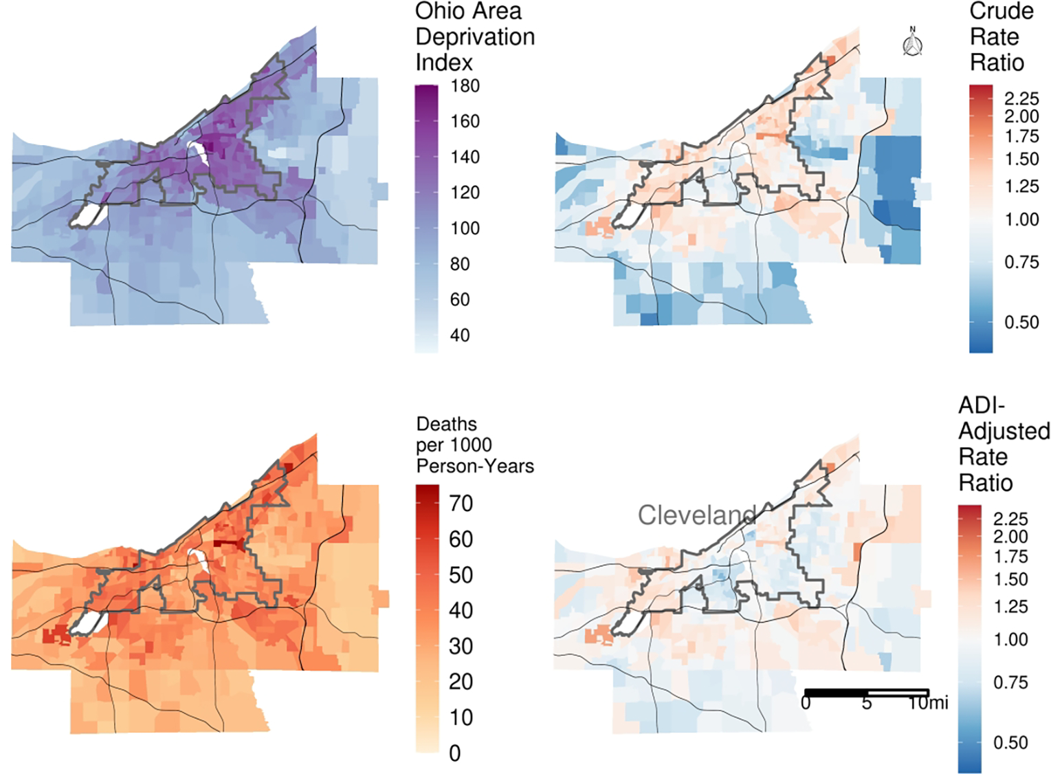
Ecological analysis of the correspondence between neighborhood socioeconomic position (Ohio Area Deprivation Index, ADI; higher values reflect greater socioeconomic disadvantage) and mortality rates in Cuyahoga County, OH. The two areas shown without data are Cleveland Hopkins International Airport to the west and industrial zoning on the banks of the Cuyahoga River in the center of the county. We used a Poisson rate model incorporating spatial autocorrelation terms to identify the rate ratios for death in the two right panels.

We estimated two log-linear (Poisson) CAR models, using the CARBayes R package²⁸, to characterize tract-level variability in death rates while accounting for correlation in outcomes among adjacent tracts. Both models were of the general form log (deaths) = log (personYears) + X′β + z_i. (Using an offset of the total number of person-years of observation allowed for directly modeling tract-specific death rates as opposed to the counts themselves.) The fixed effects coefficients β captured systematic variation in death rates associated with specific variables entered into the model. The random effects z_i = u_i + v_i captured tract-level residuals according to the Besag-York-Mollié (BYM) correlation structure: the BYM model combines spatial/structured (u_i) and unstructured (v_i) components to model residuals. The first (null) model was an intercept-only model; this model was used to describe tract-level rate ratios (as compared to the overall average across all tracts in the county). The second model incorporated (quadratic) fixed effects to model the systematic relationship between ADI and death rate.

Rate ratios (calculated for each tract as $e^{z_i}$) from these two models are given in the right two panels of Figure 4. The Figure indicates that, after adjustment for ADI, the intensity of variation among tract-level rate ratios was reduced. This can be quantified by calculating the ratio of the sum of squared residuals between the two models, i.e., $\left({\sum }_{i=1}^n{z}_{i2}^2\right)÷\left({\sum }_{i=1}^n{z}_{i1}^2\right)$, where z_i1 and z_i2 are residuals for the i^th tract from models 1 and 2 (respectively). This ratio was 0.418, meaning that 58.2% of the tract-level variation in death rates was accounted for by ADI.

Discussion

In this paper we have outlined approaches for designing and implementing analyses of EHR data for researchers interested in studying the health outcomes of individuals from diverse neighborhood environments and racial and ethnic backgrounds. Ongoing improvements in the quality, scale, and accessibility of EHR data and corresponding methodological advances provide an unprecedented opportunity for high-resolution insights into the mechanisms of social and neighborhood-level health disparities. These studies are resource-intensive to implement due to the nature of EHR data systems, which are large and complex: Special considerations are needed in the design and analysis of any study that utilizes EHR data, especially in EHR studies of health disparities.

Typically, an individual health system’s EHR data is not adequately representative of the larger community where it is located. Health systems each serve distinct populations, and populations across health systems within the same community may be heterogeneous. Therefore, efforts to understand regional health outcomes using EHR data must account for variances in demographic and socioeconomic characteristics collected within the EHR relative to those of the population(s) of interest. There are inherent limitations of EHR systems to accurately capture both biological and social characteristics. For example: i) it usually cannot be determined whether documented race and ethnicity information is self-reported or assigned by a clinician, and whether race and ethnicity is self- or clinician-assigned may systematically vary across racial and ethnic groups; ii) availability of individualized socioeconomic information (e.g., “social determinants of health” questionnaires, insurance status, or income) is limited and iii) data on adverse childhood experiences and other social risks (e.g., incarcerations, victimhood of intimate partner and other forms of interpersonal violence) are not commonly available. EHR systems nonetheless can provide larger and more representative samples of real-world patients and enable the investigation of heterogeneity in disease prevalence and treatment effects across socially-defined groups and neighborhoods.

The analytic approaches discussed in this paper vary in terms of the questions they are appropriate for studying and their complexity. We would advocate for starting with stratification and mapping approaches to identify the extent of heterogeneity in risk factors and outcomes and their respective relationships across the population. Critically, we suggest that heterogeneity should be expected rather than assumed away since there is always diversity in real-world populations. This is especially the case with EHR studies, inasmuch as they incorporate very large sample sizes and represent very diverse populations. If stratification and mapping do not demonstrate substantial variation, then it may be possible to evaluate homogeneous effects across groups.

There are additional ways to maximize the approaches outlined in this paper to improve the composition of a dataset built using EHR data. For example, sampling and weighting techniques aligned our analytic dataset with the local population by race, ethnicity and ADI quintile. Furthermore, it is possible and often appropriate to combine approaches, such as using weights in spatial models. Predictions from aspatial models (i.e., models defined on the basis of social factors but exclusive of specific neighborhood effects) can conceivably be studied at the neighborhood level via combination or weighting of individualized predictions, although there is a risk of bias in doing so: the researcher must be willing to assume that differences in social factors alone (and not individual neighborhood effects) adequately account for spatial variability. In implementing stratified and spatial analyses, researchers must take into account potential privacy concerns resulting from small cell sizes (e.g., the possibility that some census block groups may be represented by <10 patients).

Ours is not the first paper to outline approaches for creating better datasets when using EHR data. A paper by Bowler and colleagues identified techniques for using EHR data when conducting cardiovascular disease surveillance. Their suggestions are focused on data collection (e.g., measures should be recorded and obtained in a standardized way, merged correctly, and representative of the population of interest)²⁹. Rassen et al. discussed estimation of prevalence and incidence based on different lookback times for diagnoses in the EHR.³⁰ We previously published a paper in Medical Decision Making on difficulties in adapting EHRs for health services research.¹² Our approach extends these suggestions by identifying design and analysis approaches that enable researchers to better align EHRs with local populations and study heterogeneity in outcomes across neighborhoods and socially-defined populations.

Our analyses highlight the importance of including race and ethnicity and measures of socioeconomic status (e.g., ADI, education, employment, housing quality) when creating datasets to study differences in health outcomes. The health services and medical decision making research communities have recently emphasized the importance of including race and ethnicity and of naming racism and health inequity as having social origins requiring social solutions.^31,32 Numerous events and historical circumstances have led to extreme neighborhood-level disparities in wealth and socioeconomic status in the United States that have disproportionately impacted racial and ethnic minority populations.²⁷ These resource-related disparities are stubbornly persistent structures that continue to create disparate patterns of health-related risks and outcomes. Examples of phenomena that produce disparate resource level availability among neighborhoods include discrimination in housing and loan financing policies, offshoring of manufacturing jobs that previously supported small towns, gentrification of attractive neighborhoods in urbanized areas, and declining funding for public schools.²⁷ Correspondingly, access and utilization of healthcare services among low-income and minority populations have been impacted by escalating costs, consolidation in the healthcare sector, changes in insurance policies, uneven quality of health services delivery, mistrust of health institutions, and widening economic inequalities. Policies that produce unequal representation of individuals in datasets are not just historical footnotes. For example, researchers have found that Hispanic individuals have lower use of health services traceable to locally intensified Immigration Enforcement activity.^33–35 While this article addresses unequal representation in those who are included in EHR systems, it does not address differences in follow-up (or “observable person-time”^30,36) among members of diverse populations.

Social inequalities (and measures of community and individual social indicators) are interwoven and fundamental influencers of health, such that the intersection of multiple factors is rarely as simple as an additive relationship. Other challenges in understanding complex social-ecological mechanisms of health disparities include the fact that, in many cases, neighborhood-level measures are derived as an aggregation of individual responses to questions (as in the American Community Survey) while such individual characteristics are endogenous to a multiplicity of neighborhood conditions under which a person is responding to a question. For example, racial segregation is associated with an array of individual and neighborhood conditions including under- or unemployment, violent crime, and housing deterioration³⁷, all of which are associated with health declines. Yet, neighborhood level estimates of health represent an aggregation of all individuals living there and disentangling the health outcomes of subpopulations using these estimates is difficult. Therefore, careful and nuanced interpretation of identified associations is needed; researchers should (i) meticulously report how area-based measures are operationalized and (ii) acknowledge that modifying a single neighborhood environmental characteristic may not result in a reduction in health disparity even when that characteristic is associated with outcomes. Social-ecological mechanisms are complex and often inter-dependent.³⁸ Building on frameworks in computing and engineering disciplines, future work focused on data aggregation, privacy preservation and merging of multisector data resources to create simulated, Digital Twin versions of neighborhoods could provide enhanced ability to conduct robust population health analyses using EHR data resources.

Researchers seeking to understand and improve population health for all must pay attention to current and historical underlying circumstances of social policy and inequality, and how these contexts are operating to influence health care, health outcomes, and health data. In summary, regional EHR data can facilitate deeper understandings of the mechanisms underlying social health disparities which illuminate pathways to closing gaps. The methods described in this paper are intended as a starting point for better alignment of EHR-based observational research methods with the heterogeneous populations that they reflect. In many cases, it is appropriate to employ more than one of these methods. The methods offer opportunities for researchers to identify subgroups that have disparate types of risk (heterogeneous risk structures) for the same illness(es), create models to capture the variation in the effectiveness of therapies within and across subgroups and summarize disparate outcomes of interest across identified subgroups.

Highlights:

• EHR data are an abundant resource for studying neighborhood diversity and health.

• When using EHR data for these studies, careful consideration of the goals of the study should be considered in determining cohort specifications and analytic approaches.

• Causal mediation analysis, stratification and spatial analysis are effective methods for characterizing social mechanisms and heterogeneity across localized populations.

References

- 1.Cutler DM, Lleras-Muney A, Vogl T. Socioeconomic Status and Health: Dimensions and Mechanisms. Published online September 2008. doi: 10.3386/w14333 [DOI] [Google Scholar]
- 2.Chetty R, Stepner M, Abraham S, et al. The Association Between Income and Life Expectancy in the United States, 2001–2014. JAMA. 2016;315(16):1750. doi: 10.1001/jama.2016.4226 [DOI] [PMC free article] [PubMed] [Google Scholar]
- 3.Cutler DM, Landrum MB. How do the better educated do it? Socioeconomic status and the ability to cope with underlying impairment. In: Developments in the Economics of Aging. University of Chicago Press; 2013:203–248. [Google Scholar]
- 4.Zikmund-Fisher BJ. Toward transparent demographic analyses: Statement on the use and reporting of classification variables presented as measuring individual characteristics such as race, ethnicity, indigeneity, national origin, gender, sexual orientation, or socioeconomic status. Med Decis Making. 2022;42(3):277–279. [DOI] [PubMed] [Google Scholar]
- 5.Bunge M. Mechanism and Explanation. Philos Soc Sci. 1997;27(4):410–465. [Google Scholar]
- 6.Williams DR, Collins C. Racial residential segregation: a fundamental cause of racial disparities in health. Public Health Rep. 2001;116(5):404–416. [DOI] [PMC free article] [PubMed] [Google Scholar]
- 7.Green T, Venkataramani AS. Trade-offs and policy options - using insights from economics to inform public health policy. N Engl J Med. 2022;386(5):405–408. [DOI] [PubMed] [Google Scholar]
- 8.Dalton JE, Perzynski AT, Zidar DA, et al. Accuracy of Cardiovascular Risk Prediction Varies by Neighborhood Socioeconomic Position: A Retrospective Cohort Study. Ann Intern Med. 2017;167(7):456–464. [DOI] [PMC free article] [PubMed] [Google Scholar]
- 9.Goff DC, Lloyd-Jones DM, Bennett G, et al. 2013 ACC/AHA guideline on the assessment of cardiovascular risk: a report of the American College of Cardiology/American Heart Association Task Force on Practice Guidelines. J Am Coll Cardiol. 2014;63(25-A):2935–2959. [DOI] [PMC free article] [PubMed] [Google Scholar]
- 10.Saban KL, Mathews HL, DeVon HA, Janusek LW. Epigenetics and social context: implications for disparity in cardiovascular disease. Aging Dis. 2014;5(5):346–355. [DOI] [PMC free article] [PubMed] [Google Scholar]
- 11.Giurgescu C, Nowak AL, Gillespie S, et al. Neighborhood environment and DNA methylation: Implications for cardiovascular disease risk. J Urban Health. 2019;96(Suppl 1):23–34. [DOI] [PMC free article] [PubMed] [Google Scholar]
- 12.Taksler GB, Dalton JE, Perzynski AT, et al. Opportunities, Pitfalls, and Alternatives in Adapting Electronic Health Records for Health Services Research. Med Decis Making. Published online September 24, 2020:272989X20954403. [DOI] [PMC free article] [PubMed] [Google Scholar]
- 13.Shepard M Hospital Network Competition and Adverse Selection: Evidence from the Massachusetts Health Insurance Exchange. Am Econ Rev. 2022;112(2):578–615. [Google Scholar]
- 14.Kravitz RL, Duan N, Braslow J. Evidence-based medicine, heterogeneity of treatment effects, and the trouble with averages. Milbank Q. 2004;82(4):661–687. [DOI] [PMC free article] [PubMed] [Google Scholar]
- 15.Gourevitch MN, Athens JK, Levine SE, Kleiman N, Thorpe LE. City-Level Measures of Health, Health Determinants, and Equity to Foster Population Health Improvement: The City Health Dashboard. Am J Public Health. 2019;109(4):585–592. [DOI] [PMC free article] [PubMed] [Google Scholar]
- 16.Rushton G, Armstrong MP, Gittler J, et al. Geocoding in cancer research: a review. Am J Prev Med. 2006;30(2 Suppl):S16–24. [DOI] [PubMed] [Google Scholar]
- 17.Krieger NI, Wang C, Dalton JE, Perzynski AT. Sociome: Helping Researchers to Operationalize Social Determinants of Health Data. R Package Version 1.4.0 . URL: Https://Github.Com/NikKrieger/Sociome.; 2020. [Google Scholar]
- 18.Kind AJH, Buckingham WR. Making neighborhood-disadvantage metrics accessible - the neighborhood atlas. N Engl J Med. 2018;378(26):2456–2458. [DOI] [PMC free article] [PubMed] [Google Scholar]
- 19.Singh GK. Area Deprivation and Widening Inequalities in US Mortality, 1969–1998. Am J Public Health. 2003;93(7):1137–1143. [DOI] [PMC free article] [PubMed] [Google Scholar]
- 20.Berg KA, Dalton JE, Gunzler DD, et al. The ADI-3: a revised neighborhood risk index of the social determinants of health over time and place. Health Serv Outcomes Res Methodol. Published online April 19, 2021. doi: 10.1007/s10742-021-00248-6 [DOI] [Google Scholar]
- 21.Tingley D, Yamamoto T, Hirose K, Keele L, Imai K. mediation: R package for causal mediation analysis. Published online August 2014. Accessed June 22, 2022. https://dspace.mit.edu/handle/1721.1/91154?show=full
- 22.Buchanan AL, Hudgens MG, Cole SR, et al. Generalizing evidence from randomized trials using inverse probability of sampling weights. J R Stat Soc Ser A Stat Soc. 2018;181(4):1193–1209. [DOI] [PMC free article] [PubMed] [Google Scholar]
- 23.Mansournia MA, Altman DG. Inverse probability weighting. BMJ. 2016;352:i189. [DOI] [PubMed] [Google Scholar]
- 24.Bauer GR, Churchill SM, Mahendran M, Walwyn C, Lizotte D, Villa-Rueda AA. Intersectionality in quantitative research: A systematic review of its emergence and applications of theory and methods. SSM Popul Health. 2021;14:100798. [DOI] [PMC free article] [PubMed] [Google Scholar]
- 25.Wickham H, François R, Henry L, Müller K. dplyr: A Grammar of Data Manipulation. Published online 2021. https://CRAN.R-project.org/package=dplyr
- 26.Nardone A, Casey JA, Morello-Frosch R, Mujahid M, Balmes JR, Thakur N. Associations between historical residential redlining and current age-adjusted rates of emergency department visits due to asthma across eight cities in California: an ecological study. Lancet Planet Health. 2020;4(1):e24–e31. [DOI] [PMC free article] [PubMed] [Google Scholar]
- 27.Lee EK, Donley G, Ciesielski TH, et al. Health outcomes in redlined versus non-redlined neighborhoods: A systematic review and meta-analysis. Soc Sci Med. 2022;294(114696):114696. [DOI] [PubMed] [Google Scholar]
- 28.Lee D CARBayes: an R package for Bayesian spatial modeling with conditional autoregressive priors. J Stat Softw. 2013;55(13):1–24. [Google Scholar]
- 29.Bower JK, Patel S, Rudy JE, Felix AS. Addressing bias in electronic health record-based surveillance of cardiovascular disease risk: Finding the signal through the noise. Curr Epidemiol Rep. 2017;4(4):346–352. [DOI] [PMC free article] [PubMed] [Google Scholar]
- 30.Rassen JA, Bartels DB, Schneeweiss S, Patrick AR, Murk W. Measuring prevalence and incidence of chronic conditions in claims and electronic health record databases. Clin Epidemiol. 2019;11:1–15. [DOI] [PMC free article] [PubMed] [Google Scholar]
- 31.Boyd RW, Lindo EG, Weeks LD. On Racism: A New Standard For Publishing On Racial Health Inequities. Published 2020. Accessed October 22, 2021. 10.1377/hblog20200630.939347/full [DOI]
- 32.Flanagin A, Frey T, Christiansen SL, AMA Manual of Style Committee. Updated guidance on the reporting of race and ethnicity in medical and science journals. JAMA. 2021;326(7):621–627. [DOI] [PubMed] [Google Scholar]
- 33.Rhodes SD, Mann L, Simán FM, et al. The impact of local immigration enforcement policies on the health of immigrant hispanics/latinos in the United States. Am J Public Health. 2015;105(2):329–337. [DOI] [PMC free article] [PubMed] [Google Scholar]
- 34.Watson T Inside the refrigerator: Immigration enforcement and Chilling effects in Medicaid participation. Am Econ J Econ Policy. 2014;6(3):313–338. [Google Scholar]
- 35.Toomey RB, Umaña-Taylor AJ, Williams DR, Harvey-Mendoza E, Jahromi LB, Updegraff KA. Impact of Arizona’s SB 1070 immigration law on utilization of health care and public assistance among Mexican-origin adolescent mothers and their mother figures. Am J Public Health. 2014;104 Suppl 1(S1):S28–34. [DOI] [PMC free article] [PubMed] [Google Scholar]
- 36.Carnahan RM. Mini-Sentinel’s systematic reviews of validated methods for identifying health outcomes using administrative data: summary of findings and suggestions for future research. Pharmacoepidemiol Drug Saf. 2012;21 Suppl 1:90–99. [DOI] [PubMed] [Google Scholar]
- 37.Cohen DA, Mason K, Bedimo A, Scribner R, Basolo V, Farley TA. Neighborhood physical conditions and health. Am J Public Health. 2003;93(3):467–471. [DOI] [PMC free article] [PubMed] [Google Scholar]
- 38.Preiser R, Biggs R, De Vos A, Folke C. Social-ecological systems as complex adaptive systems. Ecol Soc. 2018;23(4). https://www.jstor.org/stable/26796889 [Google Scholar]