Water, Walls, and Bicycles: Wealth Index Composition Using Census Microdata

Abstract

In this study, we produce a valid and consistent variable for socioeconomic status at the household level with census microdata from ten developing countries available from the Integrated Public Use Microdata Series - International (IPUMS-I), the world’s largest census database. We use principal components analysis to compute a wealth index based on asset ownership, utilities, and dwelling characteristics. We validate the index by verifying socioeconomic gradients on school enrollment and educational attainment. Given that the availability of socioeconomic indicators varies considerably across samples of census microdata, we implement a stepwise elimination procedure on the wealth index to identify the conditions that produce an internally consistent index. Using the results of the stepwise methodology, we propose which indicators are most important in measuring household socioeconomic status. The development of the asset index for such a large archive of international census microdata is a very useful public resource for researchers.

1. Introduction

Measurement of household socioeconomic status is an important element in economic and demographic analyses. Household wealth measurements help researchers understand and estimate economic growth and inequality. As an economics concept, socioeconomic status (SES) has been approached from a variety of perspectives, starting with the univariate definition in Friedman’s 1957 permanent income hypothesis through the multidimensional poverty measures (Alkire and Foster, 2011). In economic development policy, measures of socioeconomic status allow for the identification of poor households in the allocation of anti-poverty programs or public resources. These measures are also useful as control variables in assessing the effects of variables correlated with wealth (Filmer and Pritchett, 2001). Household income or expenditures are often used as measures of socioeconomic status, but collecting data on either of these can be both challenging and costly. As a result, most demographic and household surveys that contain thorough measures of income or expenditures tend to have relatively small sample sizes. Census microdata represent a useful source for conducting social sciences research, particularly when nationally representative household surveys are not available.¹ Due to their larger scale, census microdata are more comprehensive in representing all population groups when compared to household surveys, thus providing precise estimates for statistical purposes. Nevertheless, despite the data availability and its comprehensiveness, most censuses do not collect information on income or expenditures, particularly in the case of developing countries.

To date, the Integrated Public Use Microdata Series (IPUMS) - International, at the Minnesota Population Center (University of Minnesota), has collected one of the world’s largest archives of census samples. These are publicly available (though restricted) and free to researchers. Currently, the database includes more than three hundred census samples taken from 1960 to the present from more than ninety countries around the world, representing more than 1 billion person records. The project provides access to data at the household and individual levels, including information on a wide range of population characteristics, such as basic demographic, fertility, education, occupation, migration, and others, which are systematically coded and documented across countries and time. IPUMS-International accumulates over 16,000 researchers registered to use their data, who have produced about 1,750 publications thus far. However, the lack of information on income or expenditures limits the ability of researchers to analyze socioeconomic data, or to control for wealth in regression analysis. The availability of a socioeconomic status indicator will significantly improve the functionality and applicability of census data in social and economic research, while also providing insight about relative poverty in a particular country.

In this paper, we construct an asset-based wealth index for IPUMS-International census microdata from ten developing countries using non-monetary indicators including asset ownership, utilities, and dwelling characteristics. We have two main research goals. First, we test the validity of the index in measuring household socioeconomic status, specifically for census microdata, through an application on education outcomes. Second, we attempt to resolve the issue of underlying variability of indicators across samples of census data (e.g. how many and which types of asset indicators). Using a stepwise elimination procedure, we explore the internal consistency of the index to uncover which types of assets make the most important contributions to the constructed index.

Our contributions are two-fold. Even though census microdata are widely available and include information on assets, there are no large-scale efforts to date to produce an asset-based measure of relative household wealth for censuses. We produce a valid and reliable measure of socioeconomic status that maybe widely applied in censuses available through IPUMS-International. The production and availability of the asset index is an important public good that has substantial practical implications for researchers, as a part of this public-use data archive. Secondly, it remains unclear how many and which types of indicators are necessary to generate a valid index. Our study helps to answer salient questions in economics because, despite the broad application of asset-based wealth indices, researchers have not examined the implications of limited asset information as a constraint to the construction of socioeconomic status measures. Given that the number and type of variables in each of the three asset categories (ownership of durables, utilities, and dwelling characteristics) varies considerably across census samples, a key contribution of this paper is the clarification and interpretation of data requirements to define a wealth index, using a stepwise procedure. Increasing the living standards in developing countries is a primary objective of economic development: thus, general improvement of measures of socioeconomic status brings economists closer to understanding and estimating the true effects of development policies and programs.

The paper is organized as follows: section two provides a review of the literature on asset-based wealth indices, section three covers the methods and data used, section four is a discussion of results, and section five presents some conclusions and extensions for future research. The appendices include more detailed figures and tables to support our results.

2. Literature review

2.1. Assets versus other measures of well-being

The asset-based approach to determining socioeconomic status has been widely used as a proxy measure of household wealth (Montgomery et al, 2000; Filmer and Pritchett, 1999 and 2001; Sahn and Stiefel, 2000 and 2003; McKenzie, 2005; among others). Constructing an asset index implies summarizing material well-being indicators, such as ownership of durable assets and housing characteristics, into a household score. Conceptually, the aggregation of assets translates into a stock of wealth, while other poverty indicators are conventionally estimated based on the flow of consumption necessary to obtain a determined bundle of goods (Filmer and Pritchett, 2001). More importantly, the asset-based approach produces a relative (not absolute) measure based on the household’s ranking within the wealth distribution. In this sense, Howe et al (2008) refer to wealth as determined by an asset-based index as socioeconomic position, as opposed to socioeconomic status, given that the index conveys information about relative positioning.

Why is using an index preferred to each individual asset variable? In the context of a regression, a single household wealth measure offers the advantage that it requires estimating only one parameter, rather than including each asset variable separately as a control. The interpretation of a summary measure is also more straightforward than assessing, for instance, the effect of owning a radio or having wood floors on an outcome of interest. Moreover, as discussed by Filmer and Pritchett (2001), it may be difficult to disentangle the direct effect of an individual asset on the relevant outcome (for example, having piped water on child morbidity) from its indirect effect through household wealth, based on coefficients calculated for each asset variable.

Several empirical assessments have contrasted expenditures to asset-based indices. Filmer and Pritchett (2001) compared both using large datasets from India, Indonesia, Nepal, and Pakistan. Their results show similar classifications of households by wealth quintiles with either measure and that the asset-based indices accurately predict school enrollment. Sahn and Stiefel (2003) find only moderate correlations when conducting direct comparisons of household rankings based on expenditures and asset indices with data from 12 developing countries, but they show that the latter is a valid predictor of child nutrition outcomes. Filmer and Scott (2012) worked with 11 datasets from the Living Standards Measurement Study (LSMS) to calculate seven different asset-based measures through alternative aggregation procedures. Their results indicate that inequalities in education, health care use, fertility, child mortality, and labor market outcomes using per capita expenditures or the asset-based measures are strikingly similar; not surprisingly, the authors suggest that if the goal is to explore inequalities or control for socioeconomic status, the asset-index approach may be more cost-effective.

The practical challenges of utilizing household expenditures or income as proxies for socioeconomic status suggest that the asset index provides a preferred alternative. Income and expenditure measurements are complicated to collect and error-prone, as they require lengthy questionnaires covering detailed information over various periods of time (Howe et al, 2008). Therefore, expenditures and income are often absent in nationally representative household surveys, in contrast to information on asset ownership, utilities, and dwelling characteristics that is easier to collect. Moreover, both are subject to a variety of problems such as seasonal fluctuations, recall bias, dearth of appropriate market values, and poor quality of price deflators (Falkingham and Namazie, 2002; Sahn and Stiefel, 2003; McKenzie, 2005; Lindelow, 2006). A key contribution of assets in conceptualizing socioeconomic status is their ability to reflect long-term wealth: asset data are less likely to be prone to fluctuations than consumption measurements (Lindelow, 2006), and, in response to any economic shock, households are likely to sell assets only subsequent to reducing consumption expenditures (Howe et al, 2008).

In addition, a number of studies assess the effectiveness of the asset index to identify inequalities or predict outcomes hypothesized to be associated with household socioeconomic status. In these cases, the validity of the index is determined through the economic gradient or distribution of relevant outcomes across strata of wealth. That is, individuals in the least wealthy households are expected to have worse outcomes in comparison to those classified at the other end of the wealth distribution. Several studies explored the empirical validity of the asset-based approach for education (Filmer and Pritchett, 1999 and 2001; Minujin and Bang, 2002; McKenzie, 2005; Filmer and Scott, 2012), fertility (Bollen et al, 2002, Filmer and Scott, 2012), nutrition (Sahn and Stiefel, 2003; Wagstaff and Watanabe, 2003), health service outcomes (Lindelow, 2006), as well as morbidity and mortality (Houweling et al, 2003; Filmer and Scott, 2012). Even though the evidence on the performance of the asset-based measures shows some mixed results, the overall conclusion points to the validity of the asset index approach.

Despite the wide application and empirical validity of the asset-based index, wealth rankings of households based on asset indices may have discrepancies with respect to those based on consumption expenditure (McKenzie, 2005; Montgomery et al., 2000; Sahn and Stiefel, 2003; Filmer and Scott, 2012). Asset indices exclude direct consumption of food and some non-food items (that could represent large components of household expenditures), while they include instead household public goods, such as piped water, and household private goods, like cellphones (Lindelow, 2006; Filmer and Scott, 2012). In addition, while consumption expenditures reflect relative prices or the market value of goods, a variety of methods have been used to produce the weights assigned to an item in an asset-based index, such as principal components based on the variance-covariance structure of the data (Lindelow, 2006). Shocks and random measurement error affecting expenditures tend to generate also larger discrepancies in household rankings in comparison to asset-based indices (Filmer and Scott, 2012). Previous research proposed procedures that may attenuate some of these comparability issues, such as modeling expenditures to produce regression-based weights. For instance, Filmer and Scott (2012) use predicted per capita household expenditures as an asset index, where their weights are derived from a regression with asset and housing indicators as control variables. Small Area Estimation (SAE) methods apply a similar notion to produce empirical poverty and inequality estimates for low-level geographical units. This technique uses household surveys to impute income or consumption on census microdata by identifying predictors common to both sources, which often include assets and housing characteristics (Christiaensen et al. 2012; Elbers, Lanjouw and Lanjouw 2002, 2003; Tarozzi and Deaton, 2009).

Although researchers often have no choice with respect to the information available to measure socioeconomic status, the literature reviewed in this section suggests not only that the asset index is an accepted approach but also that it may be a preferred alternative to other measures of well-being. Given the potential differences discussed between rankings based on income, expenditures, and assets, researchers should examine how using one of these measures may affect their research question.

2.2. Components of the index

The specific assets or asset types used to define the index may translate into discrepancies in household rankings. The literature has not explored this issue extensively, but it is a relevant issue given that many microdata sources have varying availability of asset variables. Filmer and Pritchett (2001) show that there is a large degree of overlap in household rankings when they use different subsets of assets in the construction of a wealth index. Based on data from the India National Family Health Survey 1992–93, the indices including all asset indicators available are compared to: a) all variables excluding drinking water and toilet facilities; b) ownership of durable assets, housing characteristics, and land ownership; and c) only durable asset ownership variables. They find that these alternative indices have high rank correlations with the index using all assets and contend that adding more variables only increases the similarity of the rankings. McKenzie (2005) uses the 1998 Mexico’s National Income and Expenditure Survey (ENIGH) to compare an index with all available assets to “specialized indices” based on differing groups: housing characteristics, access to utilities and infrastructure, and durable assets. Similarly, the study finds high correlations of the “specialized indices” with the asset-based index using all indicators and with non-durable consumption.

However, Houweling et al. (2003) show that the ranking of households and inequalities in child mortality and immunization are sensitive to the types of indicators used to construct the asset index. The study compares an index that uses all variables available for each country against alternative measures that exclude: 1) water supply and sanitation items; 2) water supply, sanitation, and housing characteristics; and 3) water supply, sanitation, housing characteristics, and electricity. The observed size and direction of changes in inequalities differ across outcomes and countries. Houweling et al (2003) suggest that inequality will decrease when the index excludes direct determinants of the outcome of interest (i.e. sanitation facilities when analyzing child mortality) or assets that are publicly provided or depend on community level infrastructure (i.e. electricity or other utilities). Moreover, the authors hypothesize that household rankings will change as items are excluded from the initial full set of available assets in the index. The remaining subset of assets is expected to be more homogenous, have higher common variance, and to more closely capture household wealth.

The availability of data only on a few or broad categories of assets owned by most of the population restricts the sensitivity of the index to capture differences across households. Moreover, data collection often captures ownership but not necessarily the quantity or quality of assets (Falkingham and Namazie, 2002; McKenzie, 2005; Vyas and Kumaranayake, 2006; Wall and Johnston, 2008), which are relevant characteristics to measure household wealth. Therefore, the index may not be able to differentiate between two types of cars, whether an appliance is in working condition, or if access to water through a public network is subject to service interruptions. Similarly, the number of items owned by a household may be relevant but not always available for assets such as cellphones, televisions, or vehicles.

Inadequate asset information may cause some concrete limitations in classifying households. Clumping and truncation have surfaced in previous research as practical data issues for asset indices. Clumping occurs when households are grouped in small numbers of clusters of measured wealth levels; this issue is commonly found in indices with a large proportion of households having similar access to public services or durable assets (McKenzie, 2005; Vyas and Kumaranayke, 2006; Howe et al, 2008). Truncation refers to a more uniform distribution of socio-economic status spread over a relatively narrow range, making it difficult to distinguish between the poor and very poor, or the rich and very rich households (McKenzie, 2005; Vyas and Kumaranayke, 2006). In this respect, Minujin and Bang (2002) state that as a necessary condition for the construction of an asset index, the indicators must be sensitive to separate households by wealth along the whole wealth distribution (including the tails).

3. Methods

3.1. Data

In this study, we used ten census samples available through IPUMS-International: Botswana 2001, Brazil 2000, Cambodia 1998, Colombia 2005, Dominican Republic 2002, Panama 1980, Peru 1993, Senegal 2002, South Africa 1996, and Thailand 2000. The data have information on a broad range of population and household variables, including household’s asset ownership, access to utilities, and dwelling characteristics. We used microdata samples from Africa, Latin America, and Asia to test our methodology across the developing world. A detailed description of the census samples and variables available for the asset index is included in Appendix 1.

After recoding data into dichotomous variables, the Botswana, Colombia, Dominican Republic, Panama, Peru, and Senegal samples have relatively more asset variables available (65+ indicators), the Brazil, South Africa, and Thailand samples are in the middle (with 43, 42, and 42 indicators, respectively) and, finally, the Cambodia sample has the fewest amount of variables (only 22). In terms of variety of indicators, the Cambodia and South Africa samples lack almost all asset ownership data, while those two samples and Brazil report just one item under dwelling characteristics. Other censuses have multiple items for asset ownership, utilities, and dwelling characteristics. The Cambodia sample is the most limited in this regard, only including fuel for cooking, fuel for lighting, water source, availability of toilet, and household members per room. Even though the dearth of diverse information about ownership of wealth indicators limits the reliability and validity of the wealth index, these samples are included as a point of comparison. A complete table showing the type and number of variables available for each sample is shown in Appendix 1.

3.2. Definition of the index

The asset-based index follows this general form: $W{I}_i=w_1{a}_{1i}+w_2{a}_{2i}+\dots +w_k{a}_{ki}$, where WI_i is the index calculated for household i, a_ji is the indicator for ownership of asset j for household i, and w_j is the weight assigned to asset j based on the first principal component (j=[1,k]). The weights to define the index are calculated through Principal Component Analysis (PCA), a data reduction technique that creates orthogonal linear combinations from a set of variables, assigning weights according to their contribution to the overall variability (Jolliffe, 2002; Rencher, 2003). In order to apply PCA to census microdata, we transform all variables into dichotomous versions, including categorical variables representing housing characteristics (e.g. material of walls or floor) or access to utilities (e.g. type of water source or sewage service). This procedure follows Filmer and Pritchett (2001) and other research in this topic.² If ownership of more than one unit of an item is reported (e.g. bicycle or television), these are recoded into binary indicators of ownership (or not) over the specific asset. While we include the “other” residual categories (for example, flooring made of some “other” type of material), we exclude missing or unknown responses.

The first principal component is assumed to represent household wealth and is used to generate a relative household score. By construction, the first component explains the maximum amount of variance retained from the indicators, relative to further components. Although it is possible that the theoretical construct of wealth is multi-dimensional, utilizing additional principal components may not be required, as they could reflect data variability associated with other features of material well-being and higher order components would need to be interpreted based on their relationship with the asset variables used in the index calculation. McKenzie (2005), for example, demonstrated empirically that while the first principal component was correlated with consumption expenditure, higher order components were not. Moreover, Howe et al (2008) argue that the objective of this kind of exercise is to define a single indicator to represent household wealth and it might be unclear what aspects of wealth are captured by additional components. Results from the calculation of the first principal component by sample are shown in Table A3 in Appendix 2. The first principal component has always eigenvalues larger than one and it explains, on average, 14.6% of the data variability.

The average proportion of households with a missing wealth index is 10.5% across all datasets, where Brazil, Dominican Republic, and Senegal have less than 2% of missing cases, in contrast to Botswana, Peru, and South Africa which have about 20% (Table A4 in Appendix 2). Vyas and Kumaranayake (2000) note that the strategy to exclude missing values may lead to lower sample sizes and potentially bias in the wealth distribution, because missing data is hypothesized to occur more often for lower SES households. We examined the characteristics of missing cases to rule out this possibility. Overall, missing cases are only slightly more rural than non-missing observations (on average, 2.4% more households are rural), while we observe generally small differences in household size, age or schooling of household members (Table A4 in Appendix 2). Furthermore, only some of these cases actually have missing information due to reporting errors, refusal, problems in data processing, or similar reasons. In fact, about 52% of households with missing information are collective or correspond to “other” types of special households that were not asked the relevant census question during data collection.³ Intuitively, persons in a hospital or a boarding school should not have household wealth defined by the characteristics of the building that they inhabit, and it is unclear whether these living arrangements would have (or not) a disproportionate representation of lower SES households. After accounting for collective and special households, the average proportion of households with a missing wealth index drops to 6.7%. Thus, the evidence suggests that the potential bias created by missing information is modest, if observed at all, in the data.

The weights produced using PCA were calculated country by country, including all households available in each census sample. Nevertheless, it has been argued that assets may have a different relationship with socioeconomic status across specific sub-groups within a population (Falkingham and Namazie, 2002; Vyas and Kumaranayake, 2006; Howe et al, 2008; Assaad et al, 2010). In particular, households residing in rural areas may be disproportionately classified as less wealthy if assets such as farmland or cattle are not appropriately weighted, given that these are atypical examples for wealth accumulation in urban areas. The complementarity of assets and housing characteristics to public infrastructure could also lead to overestimation of socioeconomic status for urban households (Filmer and Pritchett, 2001; Lindelow, 2006). We analyzed urban-rural differences, to explore whether weights may be more appropriately defined by area of residence. The wealth indices calculated by country show that there is gap in socioeconomic status for households in urban and rural areas (Table A5 in Appendix 2). On average, this gap appears to be of similar size to that observed for years of schooling of household members, while there are no significant differences in household size or age of household members. Based on this evidence, we chose to produce the wealth indices only by country for two practical reasons. The data have the disadvantage that they only include a few rural-specific assets for Botswana, Senegal, and Thailand.⁴ More importantly, the urban-rural specialized indices imply a potential loss in comparability of results across households within a country.

Finally, a natural related question is whether the index should be produced from a single pooled dataset including all countries in the study. The main advantage of this approach would be to increase the comparability of wealth indices, using common weights across countries. However, the calculation of an index from pooled data require standardizing the underlying data across census samples, so that common weights are applied to variables using the same coding structure, in addition to working only with variables available in all datasets. Even though IPUMS-International offers harmonized variables, we would lose the detailed variable categories that we are precisely trying to exploit in this study. Furthermore, the overlap in variables across countries is not substantial, as shown in Table A2 in Appendix 1, so variables available only in certain census samples would be dropped from the analysis.

3.3. Research questions

The paper focuses on two separate but interrelated questions. First, we verify the validity of the index in measuring household socioeconomic status, specifically for census microdata through an application on education outcomes. We expect education to be highly dependent on the household relative standing in the SES distribution. That is, we expect better education outcomes and statistically significant differences for higher SES as determined by the index. We first examine distributions of education enrollment and attainment by the wealth index quintiles. Then, we estimate a logit regression for school enrollment (for children aged 6 to 14 years) using the census microdata, controlling for the wealth index and other child, household, and geographic variables (odds ratios corresponding to these estimations are reported in Table 2.) The child characteristics control variables include sex, age, and age squared of the child; household characteristics include sex, age, and educational attainment dummies for the household head; geography variables include urban residence and dummies for highest level of geography for each country.

Table 2:

Logit model for Children’s School Enrollment (age 6–14), Census Wealth Index coefficient (odd-ratios)^1/

Census sample	Obs.	Model 1		Model 2		Model 3
		Odds-ratio	Pseudo R2	Odds-ratio	Pseudo R2	Odds-ratio	Pseudo R2
Botswana 20012/	25,842	1.664*** [0.0402]	0.222	1.554*** [0.0444]	0.224	1.696*** [0.0555]	0.229
Brazil 2000	1,872,876	1.935*** [0.0046]	0.125	1.798*** [0.0050]	0.132	1.967*** [0.0084]	0.142
Cambodia 1998	297,898	1.634*** [0.0088]	0.142	1.489*** [0.0082]	0.157	1.446*** [0.0103]	0.179
Colombia 2005	725,394	2.379*** [0.0106]	0.118	2.053*** [0.0103]	0.128	2.098*** [0.0137]	0.140
Dominican Republic 2002	157,448	1.129*** [0.0099]	0. 197	1.116*** [0.0111]	0.198	1.116*** [0.0137]	0.199
Panama 1980	42,913	2.553*** [0.0469]	0.167	2.246*** [0.0507]	0.173	2.070*** [0.0552]	0.175
Peru 1993	392,880	1.659*** [0.0108]	0.043	1.494*** [0.0109]	0.049	1.296*** [0.0116]	0.056
Senegal 2002	246,578	2.111*** [0.0106]	0.090	1.712*** [0.0096]	0.115	1.766*** [0.0152]	0.149
South Africa 1996	678,735	1.660*** [0.0068]	0.185	1.545*** [0072]	0.189	1.576*** [0.0112]	0.191
Thailand 2000	85,797	2.300*** [0.0675]	0.139	2.112*** [0.0663]	0.144	2.424*** [0.0862]	0.174
Child characteristics		Yes		Yes		Yes
Household characteristics		No		Yes		Yes
Geography		No		No		Yes

Data source: Minnesota Population Center, Integrated Public Use Microdata Series (IPUMS) - International.

Robust standard errors in brackets,

^***p<.01,

^**p<.05,

^*p<.10

^1/Child characteristics include sex, age, and age squared of the child; household characteristics include sex, age, and educational attainment dummies for the household head; geography variables include urban residence and dummies for highest level of geography for each country.

^2/Urban residence is not available in Botswana 2001.

The second research question addresses the conditions necessary to produce an internally consistent index. The underlying issue is the variable availability across censuses, which could have any number of items listed under each asset type. Even though the general recommendation has been to use the most variables available as long as those are related to unobserved wealth (Rutstein and Johnson, 2004; McKenzie, 2005), it remains unclear which types of assets make the most important contributions to the constructed index and how many household variables are necessary to generate a valid index.

In order to define a standard for input requirements for the index, we perform a stepwise elimination of variables (one at a time) following the order of the PCA scoring factor (from the smallest to the largest in absolute value) and recalculate the index at each step with the remaining variables. The objective of this procedure is to determine how sensitive the index is to changes in variable availability. In fact, the indicators available to construct the asset-index vary widely in the census samples used for this study. Given that PCA is based on the variance-covariance structure, it gives a higher weight to variables strongly correlated with each other and those contributing more to the total variability of the data (Rencher, 2003; Lindelow, 2006). That is, variables with smaller PCA scoring factors are those with relatively lower variation, such as an asset that nearly all or very few households own (McKenzie, 2005; Vyas and Kumaranayake, 2006). Therefore, the rationale behind eliminating first variables with smaller PCA scoring factor is that these are of limited use for differentiating households by socio-economic status.

At each step of the stepwise procedure, we verify the level of agreement of rankings through Spearman rank correlations, the internal consistency of the indices using the Cronbach’s alpha, and also re-assess validity by estimating school enrollment regressions. The Spearman rank correlation is a measure of strength of association between two variables and it allows us to check whether the households were ranked similarly to the first index at each step, from poorest to wealthiest. It is effectively calculated by comparing the difference in statistical ranks for a household using the index at step k and for the same household at step 1. Cronbach’s alpha is a measure of internal reliability that will generally increase as the inter-correlations among variables increase (Cortina, 1993). It is calculated as a function of the number of asset variables, the total variance of the asset index, and the variance of each asset variable. High values of the Cronbach’s alpha are regarded as evidence that the set of items are measuring a single underlying construct. Therefore, decreasing or increasing values will indicate the extent to which the remaining assets at each step relate to each other and to the unobserved wealth. Finally, we test whether there are changes in socioeconomic gradients based on the asset index as we reduce the availability of asset variables. We estimate school enrollment regressions at each step and analyze changes in the size of the effect of the asset index (its coefficient) and in the overall explanatory power measured by the pseudo R-squared.

4. Results

4.1. Application to education outcomes⁵

The question of validity of the asset index is concerned with verifying that the index actually measures wealth and not some other phenomenon associated with ownership of durable goods, housing characteristics, or access to utilities. This research question is analyzed through socioeconomic gradients in education outcomes, which we expect to be highly dependent on household wealth. First, we calculated differences in school enrollment and educational attainment by quintiles of the asset index. We would expect considerable differences between the top and bottom quintiles if the asset index is correctly measuring wealth.

Table 1 shows the proportion of children 6–14 years old enrolled in school by asset index quintile for all the samples examined. The figures on school enrollment by quintile using census microdata show considerable differences between the top and bottom quintile, which range between 5 percentage points in Dominican Republic and Thailand, compared to 46 percentage points in Senegal (Table 1.) Moreover, we identify a strictly increasing enrollment pattern as we move from the bottom to the top quintile for all samples analyzed. As we would expect, this same pattern is reflected in primary and secondary school completion (for persons 18 years old or more) by quintiles (Tables A6.1 and A6.2 in Appendix 3.)

Table 1:

Percent of Children’s School Enrollment (age 6–14) by census wealth index quintiles

Census sample	Obs.	Lowest quintile	2nd	3rd	4th	Highest quintile
Botswana 2001	25,842	85.1	87.3	89.0	92.1	95.6
Brazil 2000	1,872,876	86.0	92.9	95.5	97.3	98.6
Cambodia 1998	297,898	52.0	55.5	57.2	61.8	74.4
Colombia 2005	725,394	77.3	88.1	91.8	95.2	97.6
Dominican Republic 2002	157,448	82.0	84.9	85.8	86.4	86.8
Panama 1980	42,913	75.3	86.6	93.1	95.6	97.0
Peru 1993	392,880	79.8	86.3	90.5	91.7	92.8
Senegal 2002	246,578	30.5	40.5	51.0	62.5	76.9
South Africa 1996	678,735	78.4	83.3	86.6	90.9	92.1
Thailand 2000	85,797	93.4	96.1	97.0	98.0	98.9

Data source: Minnesota Population Center, Integrated Public Use Microdata Series (IPUMS) - International.

The validity of the asset index was also explored through logit regressions for school enrollment conditional on the wealth index and other individual, household, and geography variables. Regressions were estimated for children ages 6 to 14. Results are shown in Table 2. The odds-ratio column shows the odds-ratio coefficients and their standard errors for the wealth index in each sample’s regression. The first model shows the effect of the wealth index on school enrollment controlling for child characteristics only, the second model adds household characteristics, and the final specification incorporates geography to the estimation.

The odds-ratio is larger than one and statistically significant in all cases, as expected. This indicates that the measurement of wealth, as represented by the census microdata wealth index, has a positive effect on child school enrollment. For example, for a one unit increase in the value of the wealth index in the first model, we expect the odds of a child being enrolled in school to be 1.935 times higher (or an increase of 93.5%) in the Brazil 2000 census. Results are robust across models. While the values of the odds-ratios are not strictly comparable across samples, given that we measure wealth with different assets in each country, the fact that all samples and models show a positive and significant effect in predicting education enrollment is further evidence of a valid measure of household wealth.

4.2. Stepwise elimination procedure

The number and type of assets included in census microdata vary considerably across countries (see Table A2 in Appendix 1). We performed a stepwise elimination of variables to determine what assets contribute the most to the final wealth distribution. In each step, we eliminate the variable with the lowest loading coefficient in absolute value (i.e., contributing the least to the calculation of the index). Then, Cronbach’s alpha was calculated to analyze internal consistency of the remaining variables and Spearman rank correlations (with respect to the first index) to examine changes in the ordering of households given by the asset index distribution. We would expect small changes in internal consistency and rank correlations as we eliminate less meaningful variables, but greater variation and decreasing values for both measures as we eliminate variables that are more important in defining the wealth index.

The stepwise procedure was performed separately for the ten census samples used in this study. The detailed graphs showing results from the stepwise procedure for Colombia 2005 are presented in Figures 1.1 and 1.2, while the results for other samples are included in Appendix 4. Figure 1.1 shows, as expected, that Cronbach alpha is constant or increases slightly during the early variable eliminations. This is showing the small mechanical effect of removing variables with very low loading coefficients. For example, the second variable to be dropped for the Peru data was ownership of a ‘tricycle for work’ (see Table A4 in Appendix 4), which intuitively should not be a key determinant of wealth and is owned only by a small proportion of households (3.7%). In contrast, large changes in the Cronbach’s alpha during the early stages of variable removal is an indicator of a less robust internal consistency; for example, this measure increases by 12% after the third variable is removed in the Cambodia sample. The Spearman rank correlations reveal that the ordering of households by socioeconomic status is almost the same for all samples for nearly the first third of variables eliminated. In the case of Colombia, for example, we obtain similar rankings of households using all 71 variables available or a subset based on only 46, given the correlation between indices is higher than 0.999. The Cambodia sample shows again a considerable decrease in correlations even if variables with relatively lower loading coefficients are removed, which is likely explained because the index is made up of fewer variables and lacks relevant asset information.

Figure 1.1: Colombia Census 2005, Cronbach alpha and Spearman.

Data source: Minnesota Population Center, Integrated Public Use Microdata Series (IPUMS) - International.

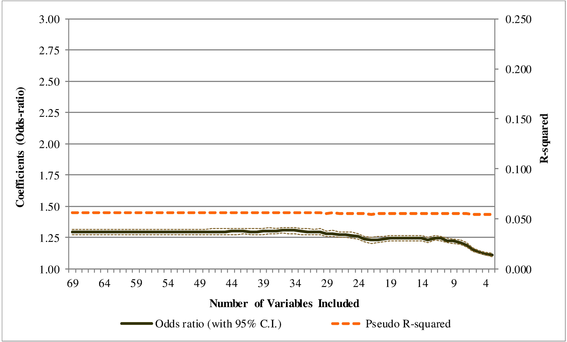
Figure 1.2: Colombia Census 2005, School enrollment regressions^1/.

Data source: Minnesota Population Center, Integrated Public Use Microdata Series (IPUMS) - International.

1/ Regressions include controls for child’s sex, age, and age squared, household head’s sex, age, and educational attainment, urban/rural status and dummies for highest level of geography for each country.

Furthermore, we observe across the majority of samples that after eliminating about two-thirds of the available variables, both internal consistency and the rank correlations begin to decrease. In the very last part of variable elimination, internal consistency may increase given we are left only with a few asset indicators that are strongly related to each other. This can be seen, for instance, in Figure 1.1 for Colombia: internal consistency starts dropping when about 25 variables are remaining. At that point, variables that have higher PCA loading coefficient in the construction of the wealth index are being removed. We also observe a sharp change in Cronbach’s alpha when a continuous variable is eliminated; for example, there is a large increase when the number of household members per bedroom is removed from the index for Colombia 2005 (index with 26 variables in Figure 1.1) and Cambodia 1998 (index with 13 variables in Figure A3.1 in Appendix 4).

Based on the stepwise procedure, we also estimated the school enrollment regressions at each step of the variable elimination process and recorded the wealth index odds-ratios and the pseudo R-squared, following the full model with child, household, and geography controls (Figures 1.2 below and A1.2 to A9.2 in Appendix 4). These figures show a relatively constant pseudo R-squared value for the most part of the variable elimination, before it begins to drop (significantly for some countries). Likewise, the odds-ratios for the wealth index are generally stable over the elimination of about one half of variables, but become less stable and start decreasing when the wealth index effects are approximated with far fewer indicators. The odds-ratios show almost consistently positive (i.e. larger than one) and statistically significant effects. Furthermore, we gain precision in the estimates for most samples as we eliminate more variables, given the reductions in the robust standard errors for the wealth index coefficient. In particular, the 95% confidence interval for the odds ratio coefficients shown in Figures 1.2 and A1.2 to A9.2 is narrower as we drop variables, even though this is difficult to observe given the small robust standard errors due to the large number of observations.

For the most part, we do not observe large changes in internal consistency, ranks, or regressions results during most of the stepwise procedure. Changes generally occur when we have only one third or less of the original set of variables available are remaining. This finding suggests that an index based on a more restricted subset of assets, dwelling characteristics, and utilities should produce results reasonably similar to those based on all variables available for each sample. However, we argue that the results demonstrate that the Cambodia sample (and to a lesser degree, the Thailand sample) lacks an adequate initial set of household variables to measure wealth. The wealth index for Cambodia was created using 22 household variables and only 42 are available for Thailand. The Cambodia index is also limited as it only includes fuel for cooking and lighting, water source, availability of a toilet, and household members per room. In turn, the Thailand sample has slightly more variables (such as walls material or type of toilet), but it includes only one variable for dwelling characteristics and lacks information on the household members per room or bedroom. This inadequacy of the Cambodia index is reflected in the irregular nature of the internal consistency and the way the household ranks change considerably. The wealth index produced by the Cambodia sample (and to a lesser degree, the Thailand sample) is a less reliable measurement of household socioeconomic status due to the limited number of variables available and the lack of key asset ownership variables. In this sense, the evidence we observe in the data analyzed suggests that having less than thirty indicator variables affects the consistency and validity of the asset-based index.

4.3. What assets are most important to define wealth?

The last subset of variables retained in the stepwise procedure gives us evidence on which assets are more important in defining the wealth index. Even though the types of variables in the final subset are slightly different for each sample, we examined the last third of variables that remain after the elimination process across the seven samples for insights into patterns arising from the indices. Part of the stepwise elimination results is presented in Table 3 below for Colombia, and Table A7 in Appendix 4, where we show the first seven and last seven indicators eliminated for each sample. The grey shading in these tables identifies the indicators that correspond to the top or bottom options for dwelling characteristics and access to utilities (excluding ‘other’), which are generally the best (i.e. wealthiest) and worst (i.e. poorest) alternatives. We opted to identify the first and last options in the analysis rather than a designation of higher or lower quality items, that may be subjective or not entirely clear for certain variables (e.g. cement, wood, or tile floor materials).

Table 3:

Colombia, first and last seven indicators eliminated^1/

Colombia 2005 (71 indicators)
Variable description	% of households
First seven indicators eliminated
Walls material: Prefabricated material	1.1
Source of water: Bottled or baged water	0.8
Fuel for cooking: Petroleum, gasln., kerosene, alcohol	0.5
Fuel for cooking: HH does not prepare food	6.2
Ship, sailboat, or boat	0.7
Toilet: Without connection, latrine, or hole, shared	0.3
Fuel for cooking: Mineral coal	0.8
Last seven indicators eliminated
Bathroom (with shower)	69.2
Connection to running water	74.9
Fuel for cooking: Wood, discarded materials, veg. coal	29.6
Source of water: Aqueduct, inside the dwelling	56.4
Trash removal: Collected by trash services	60.1
Sewage drains	57.1
Toilet: Connected to a sewage drain, exclusive	50.4

Data source: Minnesota Population Center, Integrated Public Use Microdata Series (IPUMS) - International.

^1/Shaded cells correspond to the top and bottom options from the original categorical variables (excluding ‘other’).

Based on the detailed list of variables in the stepwise process for each sample, we observe fluctuating, but clear increases in frequencies towards the last subset of assets. For instance, the first seven indicators eliminated for the Cambodia sample are reported on average by 2.9% of households, while the last seven indicators by 30% of households (Table A7 in Appendix 4). In general, assets, utilities, and dwelling characteristics with very low frequencies are less likely to contribute to the overall construct of socio-economic status and, therefore, were removed earlier in the stepwise elimination process. For example, this is the case for owning a tricycle for work in Peru (reported by 3.7% of households), having walls made of prefabricated material in Colombia (1.1%), or using solar energy for lighting in Senegal (0.8%). Intuitively, if we were creating an index using only one indicator variable, the largest variance would be achieved with an asset owned by exactly half of the country’s population. Results show that, on average, the first seven indicators eliminated were reported by only 5.9% of households across all countries, while the last seven by 44.3%.

The next clear observation about the final subset is that the bottom and top options from each categorical variable are systematically among the last variables to be removed. Across the ten census samples, the final subset of seven indicators eliminated included, on average, four top or bottom options; in contrast, the first seven indicators eliminated have only 0.6, on average. For example, the last seven variables eliminated include “flooring made of earth” for Peru and “walls made of cement” for Senegal. It is reasonable to assume that these two distinguishing indicators play a significant role in the determination of a household’s socioeconomic status, because they clearly differentiate poor from wealthy households. In addition, across all samples, the best and worst water sources and sewage or toilet types were among the most common in the final subset of variables, followed by the fuel type for cooking or lighting (which in many cases refers to household access to electricity.) Having piped water into the dwelling represents the wealthiest water source option, while water from natural sources, such as a river, rain water, or an unprotected spring represent the poorest type of water source. Similarly, a flush toilet connected to the public system contrasts with the poorest option of lacking a toilet facility. Water source appears to be an important determinant of household wealth because, in addition to having the best and worst indicators in the final third of variables, we observe that five samples had three or more water indicators among the final third of variables.

However, the final subset of variables is not exactly about the richest and poorest defining characteristics. Variables that seemingly represent extreme poverty or wealth (and tend to have low frequencies) are not included in the final subset. For example, the indicator variable for using rain water in the Thailand sample is one of the first variables removed from the index, because it has an extremely low frequency (only 1.7% of households use rain water). Further, in the Colombia sample, lacking walls completely (in response to a question about wall material) is one of the variables removed early in the stepwise procedure. This is a characteristic of extreme poverty and, in fact, 0.19% of households in Colombia lack walls. Therefore, while asset indicators that identify the very wealthy and the very poor are important for detecting the tails of the SES distribution, we observe that the wealthiest and poorest most common options within categorical variables weigh the most significantly in defining the overall index. The evidence is consistent with McKenzie (2005) who noted that principal component analysis places more weight on unequal distributions of household assets, which more precisely differentiate wealth among households. Thus, not only does the ranking of the asset indicator matter, but also the relative frequency of ownership across the population.

5. Conclusion

In this paper, we demonstrate that the census microdata wealth index is valid and internally consistent in its representation of household socio-economic status for ten IPUMS-International samples. Evidence provided by the education outcomes gradients shows that we are measuring unobserved socioeconomic status at the household level. As expected, we observe differences in school enrollment and educational attainment across the wealth index quintiles, showing that households at the top of the distribution have better outcomes than those at the bottom. The logit regressions give consistently positive and significant effects of the household wealth index on child’s school enrollment. Moreover, as we remove individual variables and re-run the regression, we see this effect is consistently positive, while predictive power is generally constant until the wealth index is comprised of too few household variables. For a majority of samples, ranks and internal consistency also remain fairly constant during most of the stepwise elimination process.

An important methodological implication arises from our results. The stepwise elimination process provides a methodology to determine which, and how many, household variables are important to include in the construction of a measurement of household socioeconomic status and, thus, are necessary to obtain a valid asset index. The fact that, after the stepwise procedure, the final subset of variables always includes the poorest and wealthiest type of water supply, sewage or toilet type categories, in addition to access to electricity, shows their value as determinants of socio-economic status. More generally, the top and bottom categories for dwelling characteristics and utilities as well as those with higher frequencies have larger contributions to the construction of a wealth index. This stepwise procedure is a robust methodology to determine which household variables are necessary in the construction of a census microdata wealth index. The results also suggest that having less than thirty indicator variables, lacking diverse asset information, or missing key variables such as water source, toilet, sewage, or electricity may negatively affect the consistency and validity of the resulting asset-based index.

Our analysis is not without limitations. The asset- based wealth index only measures wealth at the household level. Because households report assets in the census data that we examined, the index cannot differentiate wealth at the individual level. Additionally, there remain possible discrepancies in wealth rankings of households based on asset indices versus those ranked by consumption expenditure. Thus, researchers should identify and discuss the possible implications of applying this alternative SES measure to their specific research question. We also acknowledge the potential issues in comparability of results across countries, given that the calculation of PCA weights is done separately for each census sample. Finally, in our attempt to avoid relying on subjective assumptions about the ordering of categorical variables, we opted not to produce the asset-based index using polychoric correlations or ordinal asset data.

Despite these shortcomings, the release of the census microdata wealth index in publicly available IPUMS-I data will enhance social science research by providing a robust and cost-effective variable to represent socio-economic status. The index will be most applicable in developing countries, where we expect a higher variability in ownership of assets, dwelling characteristics, and access to utilities. The production and availability of the asset index is an important public good that has significant practical implications for the many researchers using IPUMS-I. This paper provides evidence of a valid census microdata wealth index in the world’s largest census database and a new methodology in evaluating which household variables are more relevant in the construction of an index.

Appendix 1: Data sources and variable availability

Table A1:

Census samples characteristics

Country	Census year	Sample characteristics1/	Sample size
Botswana	2001	10% sample, flat expansion factor	42,375 households 168,676 persons
Brazil	2000	6% sample, weighted	2,652,356 households 10,136,022 persons
Cambodia	1998	10% sample, flat expansion factor	223,513 households 1,141,254 persons
Colombia	2005	10% sample, weighted	1,054,812 households 4,006,168 persons
Dominican Republic	2002	10% sample, flat expansion factor	247,375 households 857,606 persons
Panama	1980	10% sample, weighted	47,726 households 195,577 persons
Peru	1993	10% sample, flat expansion factor	564,765 households 2,206,424 persons
Senegal	2002	10% sample, flat expansion factor	107,999 households 994,562 persons
South Africa2/	1996	10% sample, weighted	993,801 households 3,621,164 persons
Thailand	2000	1% sample, weighted	165,417 households 604,519 persons

^1/Datasets with a flat expansion factor are a systematic sample of every 10th households, including the corresponding persons in those households. The samples with a more complex design are indicated as “weighted,” however we do not use weights in our analysis.

^2/In the South Africa sample, 19 districts in Eastern Cape are not organized into households, thus individuals were treated as separate households if they reported household characteristics.

Data source: Minnesota Population Center, Integrated Public Use Microdata Series (IPUMS) - International.

Table A2:

Variable Availability in Census Samples

	Botswana 2001	Brazil 2000	Cambodia 1998	Colombia 2005	Dominican Republic 2002	Panama 1980	Peru 1993	Senegal 20021/	South Africa 1996	Thailand 2000
Durable assets
Air conditioning		X		X	X			X		X
Bicycle	X			X			X	X		X
Blender				X
Boat	X			X				2
Camera or video camera							X	X
Car or truck	3	X		X	X		3	2		X
Cart	X							X
Cistern					X
Computer	X	X		X	X		X	X
Converter					X
Electric shower				X
Fan				X						X
Floor polisher							X
Generator					X
Hot water heater				X
Knitting machine							X
Microwave		X		X
Motorcycle or scooter				X			X	2		X
Music instrument								X
Photocopy machine								X
Radio	X	X			X	X	X	X		X
Refrigerator		X		X	X	X	X	2		X
Sewing machine						X	X	2
Stereo				X			X
Stove or oven				X	X			2
Stools or canvas cover								X
Telephone or fax	X	X		X	X	X	X	2	X	X
Television	X	X		X	X	X	2	X		X
Tricycle							X
Vacuum							X
VCR or DVD player		X						X
Washing machine		X		X	X	X	X			X
Wheel barrow	X
Utilities
Water source	11	6	6	9	8	12	7	8	7	15
Sewage or waste water		7		X		7	5	9
Toilet	8	X	X	8	5	5	3	6	4	5
Waste disposal method	6	7		6	7			7	6
Electricity		X		X			X
Internet					X
Natural gas				X
Fuel used for cooking	10		7	7	5	6		5	8	7
Fuel used for heating	10								8
Fuel used for lighting	9		7		5	6		9	6
Dwelling characteristics
Housing type	11				3	7
Floor material	5			5	6	4	7	5
Wall material	9			7	6	5	8	5		5
Roof material	7				5	7	7	5
Kitchen				X	3	X	3
Members per room or bedroom	X	2	X	2	2	2	2	X	X
Access type to dwelling					5
Other
Dwelling ownership	11	6		6	5		6	7	X
Land ownership		3
Total	109	43	22	71	78	68	68	92	42	42

Data source: Minnesota Population Center, Integrated Public Use Microdata Series (IPUMS) - International.

^1/Includes durable assets corresponding to household ownership of means of production

Note: An ‘X’ indicates that the sample had this variable, while the numbers indicate the how many categories were included in each categorical variable.

Appendix 2: Wealth Index Calculation

Table A3:

Principal Component Analysis and First Component

	Botswana 2001	Brazil 2000	Cambodia 1998	Colombia 2005	Dominican Republic 2002	Panama 1980	Peru 1993	Senegal 2002	South Africa 1996	Thailand 2000
Number of indicator variables	109	43	22	71	78	68	68	92	42	42
Observations (households)	30,886	2,610,802	212,967	974,032	197,490	38,794	383,465	107,999	772,045	152,396
First principal component (index)
Eigenvalue	8.68	7.89	3.76	11.27	9.71	11.24	9.74	10.92	8.31	4.92
Proportion of variance explained (%)	7.97	18.35	17.10	15.87	12.45	16.53	14.32	11.87	19.80	11.71

Data source: Minnesota Population Center, Integrated Public Use Microdata Series (IPUMS) - International.

Table A4:

Wealth Index, Characteristics of Missing Cases

	Botswana 20011/	Brazil 2000	Cambodia 1998	Colombia 2005	Dominican Republic 2002	Panama 1980	Peru 1993	Senegal 2002	South Africa 19962/	Thailand 2000
Total households	42,375	2,652,356	223,513	1,054,812	199,143	42,965	497,550	107,999	993,801	165,417
Proportion with missing index (%)	27.11	1.57	4.72	7.66	0.83	9.71	22.93	0.00	22.31	7.87
Non-missing cases
Collective or special households (%)	0.00	0.00	0.00	0.00	0.00	0.00	0.00	0.00	0.00	0.00
Urban (%)	NA	78.99	14.56	61.43	65.53	54.33	76.17	46.75	59.48	31.51
Number of persons in household (mean)	3.97	3.85	5.17	3.83	3.91	4.64	4.70	9.21	4.16	3.70
Age of household members (mean)	28.14	31.73	24.47	32.88	30.19	28.60	28.69	24.07	29.57	33.25
Schooling of household members (mean)	6.53	5.45	2.51	5.68	5.93	5.72	6.53	2.43	6.63	6.03
Missing cases
Collective or special households (%)	15.97	100.00	65.85	0.00	100.00	78.21	18.18	NA	49.93	44.07
Urban (%)	NA	70.44	27.09	55.91	81.55	53.63	52.53	NA	62.45	57.77
Number of persons in household (mean)	4.01	2.14	3.75	3.36	1.27	3.72	3.53	NA	1.84	3.07
Age of household members (mean)	29.09	36.21	27.33	34.05	31.45	28.76	26.81	NA	30.71	32.44
Schooling of household members (mean)	3.86	4.38	3.66	5.01	6.33	4.83	5.26	NA	6.81	6.78

Data source: Minnesota Population Center, Integrated Public Use Microdata Series (IPUMS) - International.

^1/Urban or rural place of residence is not available in the Botswana 2001 census.

^2/Urban or rural place of residence is not available for collective dwellings in the South Africa 1996 census. Therefore, the proportion of urban households is calculated excluding collective dwellings.

Table A5:

Wealth Index, Urban-Rural Comparison

	Botswana 20011/	Brazil 2000	Cambodia 1998	Colombia 2005	Dominican Republic 2002	Panama 1980	Peru 1993	Senegal 2002	South Africa 1996	Thailand 2000
Total households	30,886	2,610,802	212,967	974,032	197,490	38,794	383,465	107,999	772,045	152,396
Proportion urban	NA	78.99	14.56	61.43	65.53	54.33	76.17	46.75	59.48	31.51
Urban
Wealth index (mean)	NA	0.34	1.24	0.55	0.36	0.63	0.32	0.80	0.60	0.81
Number of persons in household (mean)	NA	3.71	5.46	3.66	3.90	4.46	4.68	8.00	3.73	3.52
Age of household members (mean)	NA	32.08	24.84	33.05	29.85	28.94	28.66	25.57	31.36	33.58
Schooling of household members (mean)	NA	6.06	3.89	6.84	6.74	7.30	7.43	4.06	7.87	7.70
Rural
Wealth index (mean)	NA	−1.27	−0.21	−0.87	−0.62	−0.75	−1.03	−0.70	−0.88	−0.37
Number of persons in household (mean)	NA	4.37	5.12	4.11	3.92	4.86	4.79	10.27	4.80	3.79
Age of household members (mean)	NA	30.40	24.41	32.62	30.77	28.20	28.81	22.75	26.93	33.10
Schooling of household members (mean)	NA	3.14	2.27	3.82	4.53	3.84	3.65	0.99	4.81	5.28

Data source: Minnesota Population Center, Integrated Public Use Microdata Series (IPUMS) - International.

^1/Urban or rural place of residence is not available in the Botswana 2001 census.

Appendix 3: Education Attainment Inequalities by Wealth Quintiles

Table A6.1:

Percent of primary school completion (persons age 18 or more) by census wealth index quintiles

Census sample	Obs.	Lowest quintile	2nd	3rd	4th	Highest quintile
Botswana 2001	71,060	49.3	61.0	75.4	84.1	94.6
Brazil 2000	6,323,689	13.8	30.6	42.8	57.5	78.7
Cambodia 1998	539,291	17.6	20.3	21.8	26.7	46.3
Colombia 2005	2,268,142	31.5	48.4	62.6	75.8	89.6
Dominican Republic 2002	457,941	30.3	50.2	60.4	70.3	83.6
Panama 1980	95,874	24.8	47.4	68.4	80.7	91.2
Peru 1993	1,018,586	28.9	47.7	66.4	77.2	88.0
Senegal 2002	497,609	4.9	9.2	17.3	34.0	57.0
South Africa 1996	1,808,086	46.0	58.6	69.2	86.4	94.7
Thailand 2000	393,983	34.9	40.3	45.2	57.1	76.0

Data source: Minnesota Population Center, Integrated Public Use Microdata Series (IPUMS) - International.

Table A6.2:

Percent of secondary school completion (persons age 18 or more) by census wealth index quintiles

Census sample	Obs.	Lowest quintile	2nd	3rd	4th	Highest quintile
Botswana 2001	71,060	5.4	10.0	15.8	26.5	57.4
Brazil 2000	6,323,689	2.5	8.8	14.9	27.3	57.1
Cambodia 1998	539,291	0.7	0.9	1.0	1.6	9.9
Colombia 2005	2,268,142	5.0	12.5	23.2	35.8	61.2
Dominican Republic 2002	457,941	4.7	10.3	16.4	27.1	51.9
Panama 1980	95,874	1.0	5.1	13.7	27.7	50.4
Peru 1993	1,018,586	9.9	23.0	41.3	56.5	75.1
Senegal 2002	497,609	0.7	1.3	2.6	5.9	18.5
South Africa 1996	1,808,086	5.8	9.7	14.3	30.3	56.8
Thailand 2000	393,983	3.5	7.3	12.8	25.9	52.9

Data source: Minnesota Population Center, Integrated Public Use Microdata Series (IPUMS) - International.

Appendix 4: Stepwise Procedure

Table A7:

First and last seven indicators eliminated^1/

Botswana 2001 (109 indicators)			Brazil 2000 (43 indicators)			Cambodia 1998 (22 indicators)
Variable description	% of households		Variable description	% of households		Variable description	% of households
First seven indicators eliminated			First seven indicators eliminated			First seven indicators eliminated
Fuel for cooking: Bio gas	0.6		Trash: Placed in cleaning service bin	4.7		Light source: Other	1.3
Wall material: Wood	0.6		Land ownership: Other	2.2		Source of drinking water: Tubedpiped well	15.1
Dwelling ownership: Village Development Committee	0.8		Waste water: River, lake or ocean	2.6		Source of drinking water: Other	2.5
Fuel for cooking: Other	0.1		Dwelling ownership: Owned outright	68.7		Light source: Candle	0.2
Housing type: Shared	0.2		Dwelling ownership: Other condition	1.2		Fuel for cooking: Other	1.0
Housing type: Part of commercial building	0.2		Waste water: Other drainage	0.9		Fuel for cooking: Electricity	0.1
Housing type: Rooms	13.7		Trash: Thrown into the river, lake or ocean	0.5		Fuel for cooking: None	0.1
Last seven indicators eliminated			Last seven indicators eliminated			Last seven indicators eliminated
Fuel for heating: Wood	58.5		Water source: General system	74.2		Fuel for cooking: LPG	1.8
Fuel for heating: Electricity	8.2		Electricity	93.2		Source of drinking water: Piped water	5.8
Television	25.0		Refrigerator or freezer	81.0		Fuel for cooking: Charcoal	5.2
Fuel for lighting: Paraffin	53.5		Waste water: No bathroom or toilet	9.4		Fuel for cooking: Firewood	90.1
Fuel for lighting: Electricity	24.9		Bathroom (with shower or bathtub and toilet)	81.2		Toilet within dwelling	14.5
Water source: Piped indoors	21.2		Piped water: Piped water to at least one room	80.9		Light source: Kerosene	79.8
Toilet: Own flush toilet	26.8		Piped water: Not piped	12.1		Light source: City power	12.6
Dominican Republic 2002 (78 indicators)			Panama 1980 (68 indicators)			Peru 1993 (68 indicators)
Variable description	% of households		Variable description	% of households		Variable description	% of households
First seven indicators eliminated			First seven indicators eliminated			First seven indicators eliminated
Access type to dwelling: Other	0.3		Waste water: Communal connected to septic tank	0.9		Use of kitchen: Shared use	4.2
Floor material: Other	0.2		Fuel for lighting: Electricity from private sources	2.4		Tricycle for work	3.7
Fuel for cooking: Electricity or other	0.2		Dwelling ownership: Ceded	6.7		Walls material: Limed or cemented stone or ashlar	1.3
Dwelling ownership: Other	0.7		Fuel for lighting: Gas	0.3		Dwelling ownership: Owned, completely paid for	68.1
Waste disposal: Garbage dump	6.0		Fuel for cooking: Charcoal	0.5		Water supply: Public network, outside the dwelling	3.5
Fuel for lighting: Electricity from own generator	0.3		Water source: Outdoor public company aqueduct	19.3		Sewage: Public system, outside the dwelling	4.3
Toilet type: Shared toilet	10.3		Water source: Outdoor community public aqueduct	1.0		Dwelling ownership: used with authorization of owner	10.0
Last seven indicators eliminated			Last seven indicators eliminated			Last seven indicators eliminated
Television	68.2		Floor material: Earth	21.4		Floor material: Earth	47.7
Refrigerator	61.1		Refrigerator	44.0		Electric lighting	57.2
Stove	81.3		Television	49.1		Water supply: Public network, inside the dwelling	45.4
Fuel for cooking: Propane gas	84.0		Fuel for cooking: Gas	63.0		Sewage: Public system, inside the dwelling	37.9
Fuel for cooking: Wood	9.6		Fuel for cooking: Wood	31.3		Sanitary facilities: Exclusive use	49.9
Fuel for lighting: Public electricity	92.8		Fuel for lighting: Electricity from public company	62.8		Sewage: Does not have	36.1
Fuel for lighting: Kerosene lamp	4.5		Fuel for lighting: Kerosene	33.5		Sanitary facilities: Does not have	36.1
Senegal 2002 (92 indicators)			South Africa 1996 (42 indicators)			Thailand 2000 (42 indicators)
Variable description	% of households		Variable description	% of households		Variable description	% of households
First seven indicators eliminated			First seven indicators eliminated			First seven indicators eliminated
Type of lighting: Gas lamp	0.3		Refuse disposal: Other	0.2		Fuel for cooking: Kerosene	0.2
Sewage water disposal: Other	2.4		Fuel for heating: Other	0.1		Walls material: Wood and cement or brick	20.2
Type of lighting: Generator	0.5		Fuel for cooking: Other	0.0		Fuel for cooking: Other	0.4
Type of lighting: Solar energy	0.8		Fuel for lighting: Other	0.0		Water supply: Other	0.5
Sewage water disposal: In small river	0.2		Fuel for heating: Electricity from other source	0.2		Motorcycle	65.2
Dwelling ownership: Other	0.8		Refuse disposal: Removed by local authority less often	2.3		Water supply: Rain water	1.7
Means of production: Motorcycle, scooter, or moped	0.6		Fuel for cooking: Electricity from other source	0.2		Bicycle	42.1
Last seven indicators eliminated			Last seven indicators eliminated			Last seven indicators eliminated
Roof material: Straw or thatch	29.3		Telephone (including cellular phone)	28.4		Walls material: Cement or brick	27.6
Television	29.4		Refuse disposal: Removed by local aut. at least weekly	51.6		Motor car	25.5
Wall material: Cement	55.4		Water supply: Piped water in dwelling	43.8		Washing machine	28.7
Water source: Tap, inside the house	37.9		Toilet: Flush or chemical toilet	50.0		Telephone	28.1
Type of lighting: Electricity	40.9		Fuel for lighting: Electricity direct from authority	57.5		Air conditioner	10.4
Fuel for cooking: Wood	54.9		Fuel for cooking: Electricity direct from authority	46.9		Toilet: Flush toilet	8.2
Fuel for cooking: Gas	37.4		Fuel for heating: Electricity direct from authority	45.9		Toilet facilities: Molded bucket latrine	85.5

Data source: Minnesota Population Center, Integrated Public Use Microdata Series (IPUMS) - International.

^1/Shaded cells correspond to the top and bottom options from the original categorical variables.

Figure A1.1: Botswana Census 2001, Cronbach alpha and Spearman rank correlations.

Data source: Minnesota Population Center, Integrated Public Use Microdata Series (IPUMS) - International.

Figure A1.2: Botswana Census 2001, School enrollment regressions.

Data source: Minnesota Population Center, Integrated Public Use Microdata Series (IPUMS) - International.

Figure A2.1: Brazil Census 2000, Cronbach alpha and Spearman rank correlations.

Data source: Minnesota Population Center, Integrated Public Use Microdata Series (IPUMS) - International.

Figure A2.2: Brazil Census 2000, School enrollment regressions.

Data source: Minnesota Population Center, Integrated Public Use Microdata Series (IPUMS) - International.

Figure A3.1: Cambodia Census 1998, Cronbach alpha and Spearman rank correlations.

Data source: Minnesota Population Center, Integrated Public Use Microdata Series (IPUMS) - International.

Figure A3.2: Cambodia Census 1998, School enrollment regressions.

Data source: Minnesota Population Center, Integrated Public Use Microdata Series (IPUMS) - International.

Figure A4.1: Dominican R. 2002, Cronbach alpha and Spearman rank correlations.

Data source: Minnesota Population Center, Integrated Public Use Microdata Series (IPUMS) - International.

Figure A4.2: Dominican R. 2002, School enrollment regressions.

Data source: Minnesota Population Center, Integrated Public Use Microdata Series (IPUMS) - International.

Figure A5.1: Panama Census 1980, Cronbach alpha and Spearman rank correlations.

Data source: Minnesota Population Center, Integrated Public Use Microdata Series (IPUMS) - International.

Figure A5.2: Panama Census 1980, School enrollment regressions.

Data source: Minnesota Population Center, Integrated Public Use Microdata Series (IPUMS) - International.

Figure A6.1: Peru Census 1993, Cronbach alpha and Spearman rank correlations.

Data source: Minnesota Population Center, Integrated Public Use Microdata Series (IPUMS) - International.

Figure A6.2: Peru Census 1993, School enrollment regressions.

Data source: Minnesota Population Center, Integrated Public Use Microdata Series (IPUMS) - International.

Figure A7.1: Senegal Census 2002, Cronbach alpha and Spearman rank correlations.

Data source: Minnesota Population Center, Integrated Public Use Microdata Series (IPUMS) - International.

Figure A7.2: Senegal Census 2002, School enrollment regressions.

Data source: Minnesota Population Center, Integrated Public Use Microdata Series (IPUMS) - International.

Figure A8.1: S. Africa Census 1996, Cronbach alpha and Spearman rank correlations.

Data source: Minnesota Population Center, Integrated Public Use Microdata Series (IPUMS) - International.

Figure A8.2: S. Africa Census 1996, School enrollment regressions.

Data source: Minnesota Population Center, Integrated Public Use Microdata Series (IPUMS) - International.

Figure A9.1: Thailand Census 2000, Cronbach alpha and Spearman rank correlations.

Data source: Minnesota Population Center, Integrated Public Use Microdata Series (IPUMS) - International.

Figure A9.2: Thailand Census 2000, School enrollment regressions.

Data source: Minnesota Population Center, Integrated Public Use Microdata Series (IPUMS) - International.

References

- Alkire S; & Foster J (2011). Counting and multidimensional poverty measurement. Journal of Public Economics, 95 (7–8), 476–487. [Google Scholar]
- Assaad R; Levison D; & Zibani N (2010). The effect of domestic work on girls’ schooling: Evidence from Egypt. Feminist Economics, 16 (1), 79–128. [Google Scholar]
- Bollen K; Glanville J; & Stecklov G (2002). Economic status proxies in studies of fertility in developing countries: Does the measure matter? Population Studies, 56 (1), 81–96. [DOI] [PubMed] [Google Scholar]
- Christiaensen L; Lanjouw P; Luoto J; and Stifel D (2012). Small area estimation-based prediction methods to track poverty: validation and applications. Journal of Economic Inequality, 10 (2), 267–297. [Google Scholar]
- Cortina J (1993). What is coefficient alpha? An examination of theory and applications. Journal of Applied Psychology, 78 (1), 98–104. [Google Scholar]
- Elbers C; Lanjouw J; and Lanjouw P (2002). Micro-level estimation of welfare. Washington D.C.: World Bank, Policy Research Working Paper 2911. [Google Scholar]
- Elbers C; Lanjouw J; and Lanjouw P (2003). Micro-level estimation of poverty and inequality. Econometrica, 71 (2), 355–364. [Google Scholar]
- Falkingham J; & Namazie C (2002). Measuring health and poverty: a review of approaches to identifying the poor. London: DFID Health Systems Resource Centre. Retrieved from http://r4d.dfid.gov.uk/PDF/Outputs/HOppsIssuesPaperFalkingham.pdf [Google Scholar]
- Filmer D; & Pritchett L (1999). The effect of household wealth on educational attainment: evidence from 35 countries. Population and Development Review, 25 (1), 85–120. [Google Scholar]
- Filmer D; & Pritchett L (2001). Estimating wealth effects without expenditure data or tears: an application to educational enrollments in states of India. Demography, 38 (1), 115–132. [DOI] [PubMed] [Google Scholar]
- Filmer D; & Scott K (2012). Assessing asset indices. Demography, 49 (1), 359–392. [DOI] [PubMed] [Google Scholar]
- Houweling T; Kunst A; & Mackenbach J (2003). Measuring health inequality among children in developing countries: does the choice of the indicator of economic status matter? International Journal for Equity and Health, doi: 10.1186/1475-9276-2-8. [DOI] [PMC free article] [PubMed] [Google Scholar]
- Howe L; Hargreaves J; & Huttly S (2008). Issues in the construction of wealth indices for the measurement of socio-economic position in low-income countries. Emerging Themes in Epidemiology, doi: 10.1186/1742-7622-5-3. [DOI] [PMC free article] [PubMed] [Google Scholar]
- Jolliffe I (2002). Principal Component Analysis. New York: Springer, second edition. [Google Scholar]
- Kolenikov S; & Angeles G (2009). Socioeconomic Status Measurement with Discrete Proxy Variables: Is Principal Component Analysis a Reliable Answer? Review of Income and Wealth, 55 (1) 1, 128–165. [Google Scholar]
- Lindelow M (2006). Sometimes more equal than others: how health inequalities depend on the choice of welfare indicator. Health Economics, 15 (3), 263–279. [DOI] [PubMed] [Google Scholar]
- Lovaton Davila, Rodrigo. (2015). Testing Alternative Aggregation Methods Using Ordinal Data for a Census Asset-Based Wealth Index, Population Association of America, San Diego, CA, April 30-May 2. [Google Scholar]
- McKenzie D (2005). Measuring inequality with asset indicators. Journal of Population Economics, 18 (2), 229–260. [Google Scholar]
- Minnesota Population Center. Integrated Public Use Microdata Series, International: Version 7.3 [dataset]. Minneapolis, MN: IPUMS, 2020. 10.18128/D020.V7.3 [DOI] [Google Scholar]
- Minujin A; & Bang J (2002). Indicadores de inequidad social. Acerca del uso del ‘índice de bienes’ para la distribución de los hogares. Desarrollo Económico, 42 (165), 129–146. [Google Scholar]
- Montgomery M; Gragnolati M; Burke K; & Paredes E (2000). Measuring living standards with proxy variables. Demography, 37 (2), 155–174. [PubMed] [Google Scholar]
- Rencher AC (2003). Principal component analysis. In: Rencher AC, Methods of Multivariate Analysis (pp. 380–407), Second Edition. New York: John Wiley and Sons. [Google Scholar]
- Rutstein SO; & Johnson K (2004). The DHS wealth index. Maryland: MEASURE DHS, ORC Macro, DHS Comparative Reports No. 6. Retrieved from http://dhsprogram.com/pubs/pdf/CR6/CR6.pdf [Google Scholar]
- Sahn D; & Stifel D (2000). Poverty comparisons over time and across countries in Africa. World Development, 28 (12), 2123–2155. [Google Scholar]
- Sahn D; & Stiefel D (2003). Exploring alternative measures of welfare in the absence of expenditure data. Review of Income and Wealth, 49 (4), 463–489. [Google Scholar]
- Tarozzi A; & Deaton A (2009). Using census and survey data to estimate poverty and inequality for small areas. Review of Economics and Statistics, 91 (4), 773–792. [Google Scholar]
- Vyas S; & Kumaranayake L (2006). Constructing socio-economic status indices: how to use principal components analysis. Health Policy and Planning, 21 (6), 459–468. [DOI] [PubMed] [Google Scholar]
- Wagstaff A; & Watanabe N (2003). What difference does the choice of SES make in health inequality measurement? Health Economics, 12 (10), 885–890. [DOI] [PubMed] [Google Scholar]
- Wall M; & Johnston D (2008). Counting heads or counting televisions: Can asset-based measures of welfare assist policy-makers in Russia? Journal of Human Development, 9 (1), 131–147. [Google Scholar]