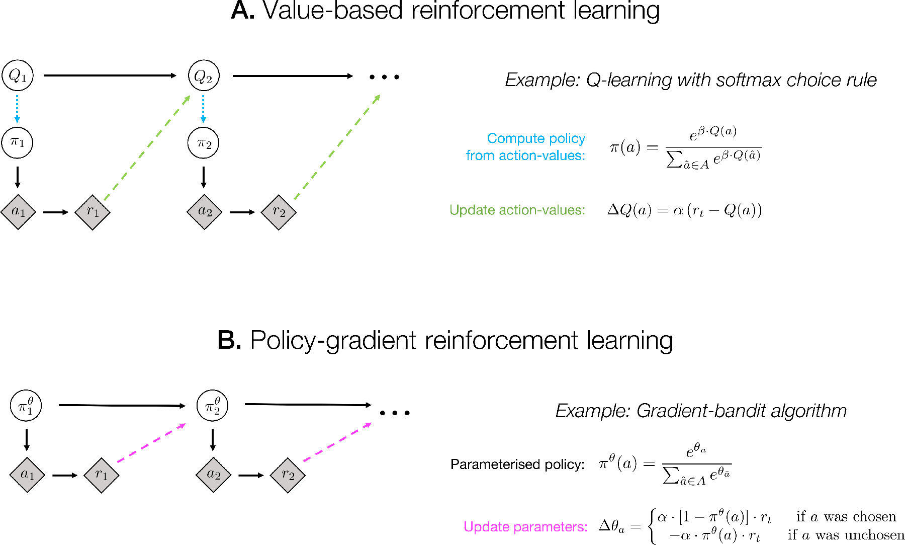
Figure 1:

Update schematics for example value-based and policy-gradient RL algorithms. Shaded diamond nodes denote observable variables, unshaded circular nodes denote latent variables that are internal to the RL agent, and arrows denote dependencies. For simplicity, in these algorithms we do not show the environmental state, which would be an additional (potentially partially) observable variable. A: in a value-based RL algorithm (such as the Q-learning model presented here), actions (a, chosen from a discrete set A) are a product of the agent’s policy π, which in turn is determined (dotted cyan arrow) by the learned action-values (Q). The update rule for action-values (dashed green arrow) depends on the action-values and received reward (r) at the previous timestep, and only indirectly on the policy. This algorithm has two adjustable parameters: the learning rate α and the softmax inverse temperature β. B: a policy-gradient algorithm (such as the gradient-bandit algorithm presented here; see [13]) selects actions according to a parameterised policy π^θ, and updates the parameters θ of this policy directly (dashed magenta arrow; in the gradient-bandit algorithm, θ is a vector of action preferences), without the intermediate step of learning action-values. In the policy-gradient algorithm, by contrast with the value-based algorithm, the size of the update to θ depends more directly on the current policy, since the size of the update to each action preference is scaled by the probability of that action under the policy.