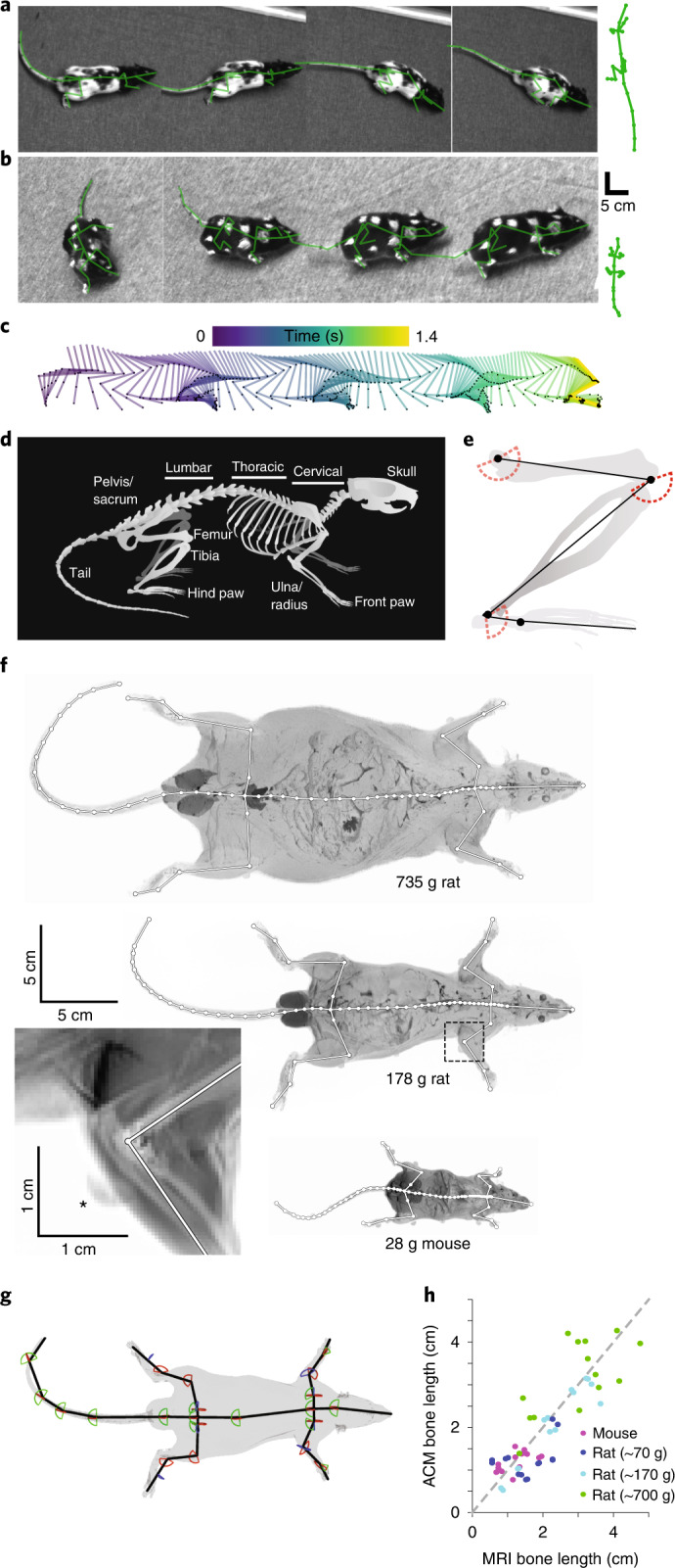
Fig. 1. Learning an anatomically constrained skeleton model for mice and rats.

a, Example images of a freely moving rat with painted surface labels, also showing the fitted and re-projected skeleton model (green). Scaled skeleton shown at right for comparison with b. b, as for a, but showing images from a freely moving mouse. Scaled skeleton on right for comparison with a. c, Time series of the reconstructed right hind limb during the sequence shown in a. d, Schematic image of a rat skeleton showing anatomical landmarks. e, Schematic image of a hind limb with modeled bones (black lines) and joints (black dots) as well as enforced joint angle limits for flexion and extension (red dashed lines). f, MRI scans (maximum projection) of two rats of different weights (top, middle), a mouse (bottom) and an enlargement of the right elbow joint from a rat (bottom left, mean projection, area denoted by dashed box) with manually labeled bone (white lines) and joint (white dots) positions. Note visible MRI surface marker (asterisk). g, 3D representation of a rat’s MRI scan showing the animal’s surface (gray) and the aligned skeleton model (black lines) and joint angle limits for flexion or extension (red lines), abduction or adduction (green lines) and internal or external rotation (blue lines). h, Learned bone lengths compared to MRI bone lengths (n = 6 rats and 2 mice). Colors represent mouse data (magenta) and small (blue, 71 g and 72 g), medium (cyan, 174 g and 178 g) and large (green, 699 g and 735 g) rat data.