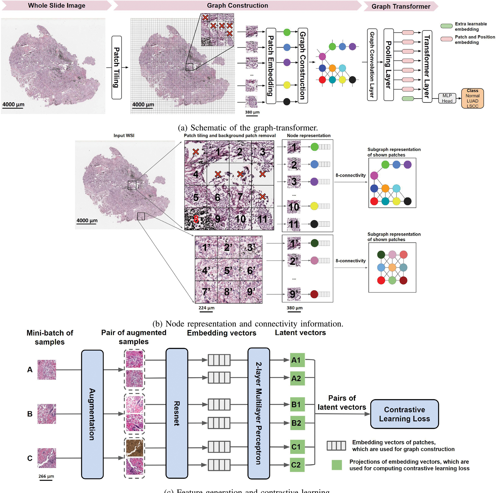
Fig. 1. The GTP framework.

(a) Each whole slide image (WSI) was divided into patches. Patches that predominantly contained the background were removed, and the remaining patches were embedded in feature vectors by a contrastive learning-based patch embedding module. The feature vectors were then used to build the graph followed by a transformer that takes the graph as the input and predicts WSI-level class label. (b) Each selected patch was represented as a node and a graph was constructed on the entire WSI using the nodes with an 8-node adjacency matrix. Here, two sets of patches of an WSI and their corresponding subgraphs are shown. The subgraphs are connected within the graph representing the entire WSI. (c) We applied three distinct augmentation functions, including random color distortions, random Gaussian blur, and random cropping followed by resizing back to the original size, on the same sample in a mini-batch. If the mini-batch size is K, then we ended up with 2 × K augmented observations in the mini-batch. The ResNet received an augmented image leading to an embedding vector as the output. Subsequently, a projection head was applied to the embedding vector which produced the inputs to contrastive learning. The projection head is a multilayer perceptron (MLP) with 2 dense layers. In this example, we considered K = 3 samples in a minibatch (A, B & C). For sample A, the positive pairs are (A1, A2) and (A2, A1), and the negative pairs are (A1, B1), (A1, B2), (A1, C1), (A1, C2). All pairs were used for computing contrastive learning loss to train the Resnet. After training, we used the embedding vectors (straight from the ResNet) for constructing the graph.