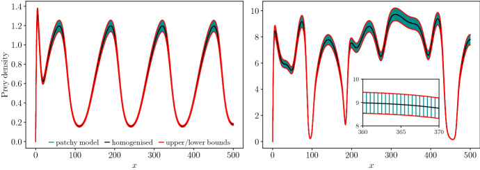
Fig. 2.

Comparison between the simulations of the patchy landscape model (blue, Eqs. 1, 2, 4) and the homogenised approximation (black, Eq. 5) prey (U) population densities. The upper and lower bounds are obtained through ${\rho }_1^{u}U/⟨{\rho }^u⟩$ and ${\rho }_2^{u}U/⟨{\rho }^u⟩$. Left (stable PTW): $t=450$, $m_1=m_2=0.8,{\mu }_1={\mu }_2=5.0$. Right (unstable PTW): $t=50$, $m_1=m_2=1.5,{\mu }_1={\mu }_2=1.0$. Initial conditions for the homogenised model are $U(x,0)=4(1+sin(2\pi x/500))$ for the prey and $V(x,0)=2(1+sin(2\pi x/500))$ for the predator. The corresponding prey initial conditions for the patchy landscape model were ${\rho }_1^{u}U(x,0)/⟨{\rho }^u⟩$ in patch type 1 and ${\rho }_2^{u}U(x,0)/⟨{\rho }^u⟩$ in patch type 2. Analogous conditions are used for the predator (V). Boundary conditions: zero-Dirichlet at $x=0$ and zero-flux at $x=500$. Other parameters: $D_1^u=21,D_2^u=19,D_1^v=22,D_2^v=20$, $l_1=l_2=0.5$, ${\alpha }^u={\alpha }^v=0.5$, $a_1=a_2=3.0,\gamma =0.9,h_1=h_2=0.5,{\lambda }_1={\lambda }_2=10.$ The numerical simulations are carried out using the method described in Yurk and Cobbold (2018). The Strang splitting is applied, with diffusion terms implemented with Crank–Nicholson and fourth-order Runge–Kutta to update the kinetic step. For the patchy landscape model, derivatives that appear in the patch interface conditions were implemented using second-order forward or backward difference. Discretisation: $\mathrm{\Delta }t=0.001,\mathrm{\Delta }x=0.1$ (Color Figure Online)