Fig. 5.

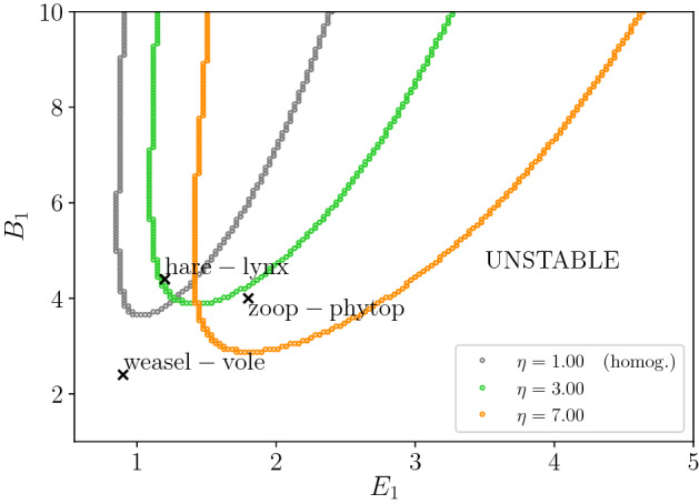
Stability boundaries in terms of the dimensionless parameters $E_1$, $B_1$ for different $\eta$, for $\beta =1.0$ when C is close to $C_{\text{crit}}$. The areas above the curves correspond to parameter regions where the PTW solutions are stable. The regions below each curve correspond to unstable PTW solutions. We plot with respect to $B_1$ (prey/predator maximum birth rate) and $E_1$ (predator birth/death rate) so that in the limiting case ($\eta =1.0$ corresponding to spatial homogeneity) we obtain the corresponding stability boundary discussed by Sherratt et al. (2003). The crosses denote the parameter sets given by Sherratt (2001) for three example predator–prey systems: hare-lynx, zooplankton-phytoplankton and weasel-vole (Color Figure Online)