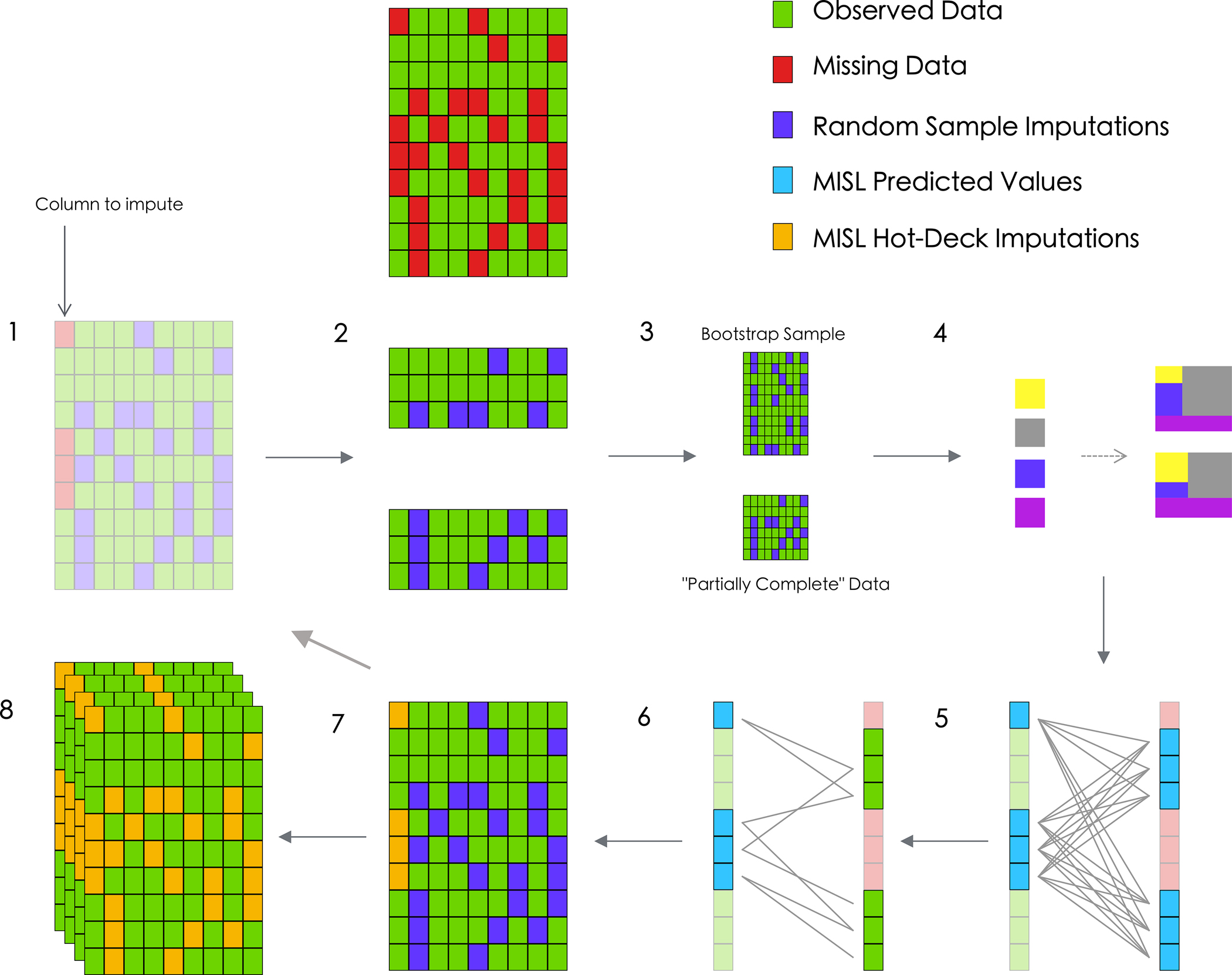
Figure 2:

Diagram of the proposed MISL algorithm for a numeric variable. MISL first isolates a random column with missing data and further draws random samples as placeholders for each subsequent incomplete column (1). The algorithm then isolates rows for which data is observed for this column (2) and generates (3) a bootstrap sample from this subset data frame (top) while retaining the “partially complete” data with respect to that column (bottom). Super learner then generates an ensemble (4) predicting the column of interest conditionally using the remaining columns available in the data for both the bootstrap sample (top) and partially complete data (bottom). MISL then generates a distance metric among each of the super learner predictions (the missing values are predicted with the bootstrap super learner (left) and observed values are predicted with the partially complete data (right)) (5). For each MISL prediction, a set of corresponding candidates from the observed data are identified based on a distance metric (6). For each missing value, MISL randomly samples one of the candidate donors and imputes this value (7). The algorithm then continues with the next column containing incomplete data and begins imputation using the newly imputed MISL hot-deck imputations (2–7). Once all columns have been imputed, the algorithm iterates M times until convergence is reached in imputations. What results is a single completed dataset; the algorithm then continues m-1 more times (8) until m distinct (full) datasets are complete.